
Overcoming catastrophic forgetting by incremental moment matching
Contents
- Abstract
- Introduction
- Previous works on Catastrophic Forgetting
- Ensemble of NN
- Implicit distributed storage of information
- Regularization Term
- Incremental Moment Matching
- mean-IMM
- mode-IMM
- Transfer Techniques for IMM
- Weight Transfer
- L2-Transfer
- Drop Transfer
- Conclusion
0. Abstract
Catastrophic Forgetting
- 새로운 task 학습 과정에서 이전 task 성능 떨어짐 ( weight 손상 )
이 논문은 CF를 극복하기 위한 IMM(Incremental Moment Matching)을 제안함
Neural Network를 task에 대해 “각각” 학습한 뒤, 이를 MoG(Mixture of Gaussian)으로 합침!
Posterior parameter의 search space를 smooth하게 하기 위해…
- 1) Weight Transfer
- 2) L2-Norm
- 3) Variant of Dropout
을 사용한다!
1. Introduction
Catastrophic forgetting은 SGD를 사용하는 모델에서 빈번히 일어나는 문제…
이를 풀고자 하는 continual learning!
최근 들어, REGULARIZATION function을 적용하는 concept이 유행함.
-
ex 1) Learning without Forgetting (LwF)
-
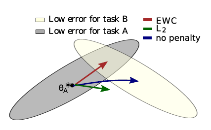
ex 2) Elastic Weight Consolidation (EWC)
( https://seunghan96.github.io/cont/study/study-(continual)(paper-2)Overcoming-Catastrophic-Forgetting-in-NN/ 참고하기! )
이 논문은 EWC의 variant version으로 볼 수 있다!
Incremental Moment Matching (IMM)
-
Bayesian NN의 framework를 사용한다
( 즉, weight에 uncertainty 부여! weight의 posterior를 계산한다 )
-
approximate MoG(Mixture of Gaussian) posterior
- 각각의 Gaussian은 각각의 task의 NN weight의 posterior
-
서로 다른 posterior를 merge하기 위해, 2가지 MM(moment matching) 방법 사용
- 1) mean-IMM
- 단순히 2 NN의 parameter를 average
- 2) mode-IMM
- Laplace approximation 사용해서 mode를 approximate
- 1) mean-IMM
사실 weight를 Gaussian으로 보는 것 자체가 너무 naive
따라서, 아래의 3 transfer learning task를 제안함
- 1) weight transfer
- 2) L2 norm of old&new task
- 3) 새롭게 제안한 variant of dropout
2. Previous works on Catastrophic Forgetting
Catastrophic Forgetting을 해결하기 위한 3가지 큰 방법들
- 1) Ensemble of NN
- 2) Implicit distributed storage of information
- 3) Regularization term
2-1. Ensemble of NN
-
새로운 task올 때마다, 새로운 NN을 형성
-
ex) Progressive NN
( https://seunghan96.github.io/cont/study/study-(continual)(paper-1)-Progressive-Neural-Network/ 참고! )
-
당연히 complexity issue…. task 수 늘어남에 따라 늘어나게 되는 network의 개수
2-2. Implicit distributed storage of information
- make use of large capacity of NN
- 하지만, extreme change of environment 상황에서는 bad
- 이에 대한 대안으로 제안된 PathNet
- extend the idea of ensemble approach for parameter reuse within a SINGLE network
- 알고리즘 간단 소개
- layer 별 10~20개의 module
- task 별로, layer별로 3~4개의 module을 pick
- complexity issue어느 정도 해결!
2-3. Regularization Term
-
앞서 말했듯, 대표적인 2개의 예시
-
1) LwF (Learning without Forgetting)
-
2) EWC (Elastic Weight Consolidation)
-
-
[LwF 간단 요약]
-
pseudo-training data from old task를 사용한다
-
새로운 task학습 이전에, 새로운 task의 데이터를 old task NN에 넣는다.
거기서 나온 output을 pseudo-label로 사용!
-
new task NN은 아래의 2개의 데이터로 학습
- new task data
- old task pseudo-training data
-
-
[EWC 간단 요약]
-
이전 task로 인해 학습된 posterior distn은, new prior를 update하는데 있어서 사용됨
이 new prior는 new posterior를 learning하는데에 있어서 사용됨
-
posterior의 covariance matrix가 diagonal 하다고 가정 ( no correlation )
하지만 그럼에도 불구하고 well working!
-
3. Incremental Moment Matching
Moments of posterior distn are matched INCREMENTAL way
[ 알고리즘 개요 ]
-
posterior를 Gaussian으로 근사함
-
\(K\)개의 sequential한 task가 있을 때, 아래의 Gaussian의 parameter들을 찾고자함
- 1) mean param : \(\mu_{1: K}^{*}\)
- 2) cov param : \(\Sigma_{1: K_{-}}^{*}\)
from each \(k\)th task \(\left(\mu_{k}, \Sigma_{k}\right)\)
\(\begin{gathered} p_{1: K} \equiv p\left(\theta \mid X_{1}, \cdots, X_{K}, y_{1}, \cdots, y_{K}\right) \approx q_{1: K} \equiv q\left(\theta \mid \mu_{1: K}, \Sigma_{1: K}\right) \\ p_{k} \equiv p\left(\theta \mid X_{k}, y_{k}\right) \approx q_{k} \equiv q\left(\theta \mid \mu_{k}, \Sigma_{k}\right) \end{gathered}\).
Dimension
- \(\mu_k\) & \(\mu_{1:k}\) : \(D\) 차원
- \(\Sigma_k\) & \(\Sigma_{1:k}\) : \(D \times D\) 차원
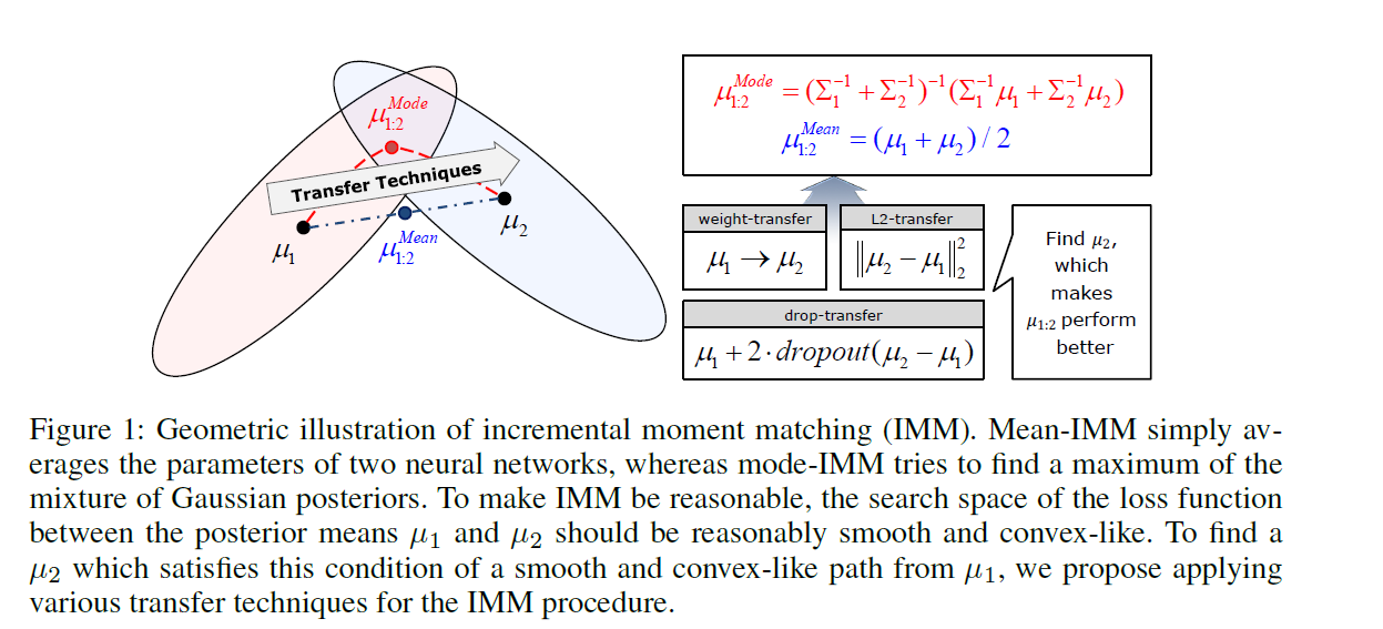
3-1. mean-IMM (Mean-based Incremental Moment Matching)
-
두 개의 NN의 layer 별로 parameter를 (weighted) average 함 ( weight : \(\alpha_k\) )
-
objective function of mean-IMM :
( 다음의 local KL-divergence를 minimize한다 )
\(\mu_{1: K}^{*}, \Sigma_{1: K}^{*}=\underset{\mu_{1: K}, \Sigma_{1: K}}{\operatorname{argmin}} \sum_{k}^{K} \alpha_{k} K L\left(q_{k} \mid \mid q_{1: K}\right)\).
-
위 문제를 풀면… optimal solution :
- \(\mu_{1: K}^{*}=\sum_{k}^{K} \alpha_{k} \mu_{k}\).
- \(\Sigma_{1: K}^{*}=\sum_{k}^{K} \alpha_{k}\left(\Sigma_{k}+\left(\mu_{k}-\mu_{1: K}^{*}\right)\left(\mu_{k}-\mu_{1: K}^{*}\right)^{T}\right)\).
-
하지만 여기서 covariance matrix는 필요 없음
-
shallow NN에서는 자주 사용되어왔다. 이 paper는 DNN에도 적용가능함을 잘 보여줌
3-2. mode-IMM (Mode-based Incremental Moment Matching)
- mean-IMM과 달리, covariance information을 사용한다
- [key idea] posterior를 maximize하는 mode를 찾자!
- mode of MoG with K cluster는 항상 \((K-1)\) dimension의 hypersurface에 존재한다!는 사실을 이용
Laplace Approximation
\(\log q_{1: K} \approx \sum_{k}^{K} \alpha_{k} \log q_{k}+C=-\frac{1}{2} \theta^{T}\left(\sum_{k}^{K} \alpha_{k} \Sigma_{k}^{-1}\right) \theta+\left(\sum_{k}^{K} \alpha_{k} \Sigma_{k}^{-1} \mu_{k}\right) \theta+C^{\prime}\).
Optimal Solution:
-
\(\mu_{1: K}^{*}=\Sigma_{1: K}^{*} \cdot\left(\sum_{k}^{K} \alpha_{k} \Sigma_{k}^{-1} \mu_{k}\right)\).
-
\(\Sigma_{1: K}^{*}=\left(\sum_{k}^{K} \alpha_{k} \Sigma_{k}^{-1}\right)^{-1}\).
( Diagonal Covariance를 가정해서, complexity를 \(O(D^2) \rightarrow O(D)\)로 축소! )
( inverse of Fisher Information matrix를 사용한다 )
4. Transfer Techniques for Incremental Moment Matching
일반적으로 NN의 loss function는 non-convex하다.
그렇기 때문에, (당연한거겠지만) 두 NN의 weight를 단순 평균때린게 잘 working할 것이라고 기대할 수 없다!
HOWEVER, 이 논문은 위 문제를 해결하기 위해 다양한 transfer learning technique를 제안한다.
4-1. Weight Transfer
- 이전 task의 weight를 새로운 task의 initial value로써 사용
4-2. L2-Transfer
\(\log p\left(y_{k} \mid X_{k}, \mu_{k}\right)-\lambda \cdot \mid \mid \mu_{k}-\mu_{k-1}\mid \mid_{2}^{2}\).
- variant of L2-regularization
- EWC의 special case로 볼 수 있음
- prior : Gaussian, with \(\lambda I\) as covariance matrix
- 여기서 사용되는 regularization term은 \(\mu_k\) 와 \(\mu_{k-1}\)의 distance
일반적으로, transfer/continual learning에서는 large \(\lambda\)를 사용하지만,
여기 IMM에서는 small \(\lambda\)를 사용한다
4-3. Drop-transfer
- 이 paper에서 제안한 새로운 방법
- 기존 dropout에서, node를 끄면 zero가 되지만, 여기서는 \(\mu_{k-1}\)이 된다
5. Conclusion
4개의 contribution
-
1) mean-IMM을 continual learning of modern DNN에 ㅈ적용
-
2) mean-IMM을 mode-IMM으로 확장
( mode-IMM이 더 성능 good…. covarinace 까지 계산해야한다는 점이 있지만 )
-
3) drop-transfer를 제안
-
4) 그 외의 다양한 transfer technique들을 적용함