[meta] (paper 3) Towards a Neural Statistician

Towards a Neural Statistician

Contents

1. Abstract
2. Introduction
3. Problem Statement
4. Neural Statistician
   1. VAE
   2. Basic Model
   3. Full Model
   4. Statistic Network

0. Abstract

효율적인 learner란?

• 이전에 습득한 지식을, 다음 task를 푸는데에 있어서 사용할 줄 아는 learner!
• 다른 말로 하면, similarities amongst datasets를 잘 아는 것!
• 관점의 전환)
  • work with data points (X)
  • work with datasets (O)

여기서 제안한 network는, statistics를 produce하도록 학습됨!

1. Introduction

summarizing datasets = Statistics (통계량)

Statistic network

• input ) set of vector
• output ) vector of SUMMARY statistics
  • ex) Normal의 mean & variance
• 이 모델의 장점
  • 1) Unsupervised
    • VAE의 output을 summary statistic로 사용
  • 2) Data Efficient
    • 적은 양의 dataset 여러 개 있을 경우?
    • model the datasets JOINTLY
  • 3) Parameter Efficient
    • summary statistic 사용하여 param 수 줄여!
  • 4) Capable of few-shot learning
    • 데이터셋들이 서로 다른 class일 경우, class embedding 사용

2. Problem Statement

Notation

• \(D_{i}\) : dataset ( where \(D_{i}=\left\{x_{1}, \ldots, x_{k_{i}}\right\}\) )
• 위 dataset의 분포 : \(p_{i}\)

Task는 둘로 나뉨

• (1) learning

  • produce a generative model \(\hat{p_i}\) for each dataset \(D_i\)

  • dataset들 내에, common underlying generative process \(p\)가 있다고 가정

    ( \(p_{i}=p\left(\cdot \mid c_{i}\right)\) for \(c_i\) , which is drawn from \(p(c)\) …. 여기서 \(c\) 는 context )

• (2) inference

  • “approximate posterior” over the context \(q(c \mid D)\)
  • 이 posterior는 Statistic Network를 통해서 얻음

3. Neural Statistician

• VAE 모델의 확장판

3-1. VAE

VAE 간단 소개

• latent variable model

• decoder : \(p(x \mid z ; \theta)\)

• likelihood : \(p(x)=\int p(x \mid z ; \theta) p(z) d z\)

  여기서 generative param인 \(\theta\)는 recognition network(encoder) \(q(z \mid x ; \phi)\) 를 통해 생성됨

  이 recognition network는 approximate posterior over latent variable를 반환함

• ELBO ( 하나의 data에 대해 )

  • \[\log P(x \mid \theta) \geq \mathcal{L}_{x}\]
  • \[\mathcal{L}_{x}=\mathbb{E}_{q(z \mid x, \phi)}[\log p(x \mid z ; \theta)]-D_{K L}(q(z \mid x ; \phi) \| p(z))\]
  • 이 ELBO를 \(\theta\)와 \(\phi\)에 대해 update

Model Architecture

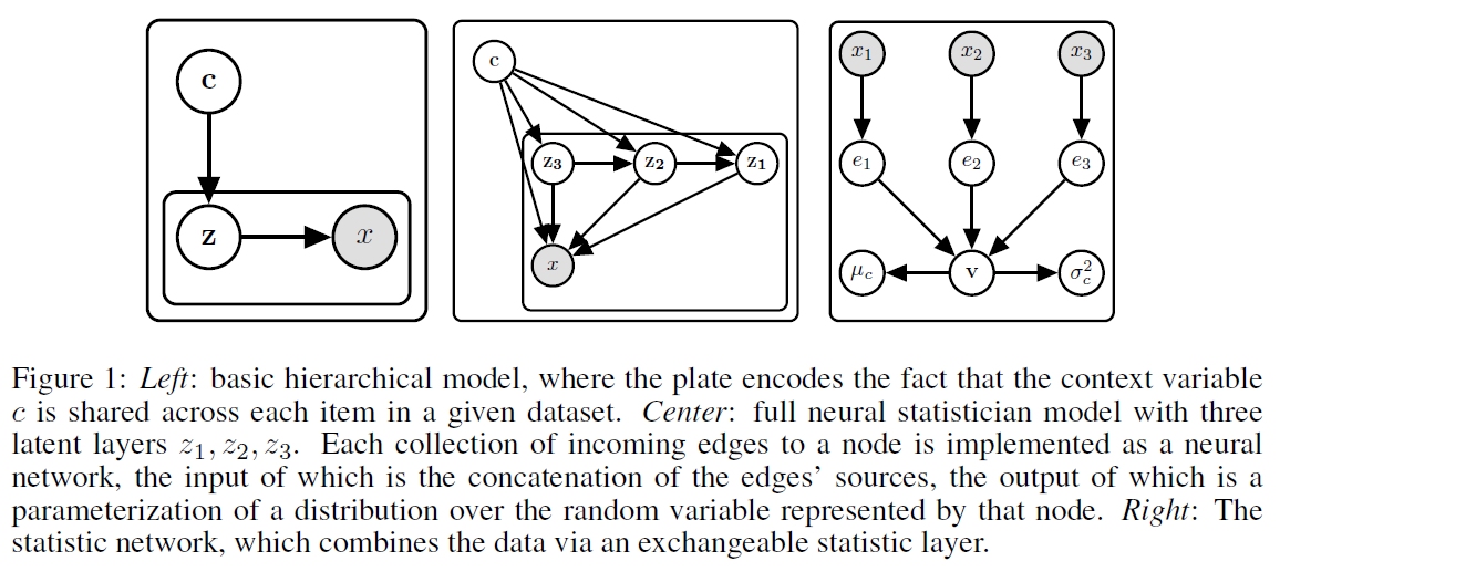
3-2. Basic Model

Likelihood for 1 data”set” :

• \[p(D)=\int p(c)\left[\prod_{x \in D} \int p(x \mid z ; \theta) p(z \mid c ; \theta) d z\right] d c\]

notation

• prior : \(p(c) = N(0,I)\)
• conditional : \(p(z \mid c ; \theta)\)
  • Gaussian with diagonal covariance
  • mean and variance parameters depend on \(c\) through NN

• observation model : \(p(x \mid z ; \theta)\)

  • 마찬가지로 NN으로 구성

• Approximate inference network : \(q(z \mid x, c ; \phi)\)와 \(q(c \mid D ; \phi)\)

• single dataset ELBO :

  \[\mathcal{L}_{D}=\mathbb{E}_{q(c \mid D ; \phi)}\left[\sum_{x \in d} \mathbb{E}_{q(z \mid c, x ; \phi)}[\log p(x \mid z ; \theta)]-D_{K L}(q(z \mid c, x ; \phi) \| p(z \mid c ; \theta))\right] -D_{K L}(q(c \mid D ; \phi) \| p(c))\]

  ( 위의 ELBO를 모든 dataset에 대해 더하면, full-data variational bound )

3-3. Full Model

위의 basic모델은 simple dataset에는 잘 working하나, data가 complex internal structure가질 경우는…?

모델의 복잡도를 높이기 위해 …

• 1) multiple stochastic layers \(z_1 ,..., z_k\)

• 2) skip-connection 사용

  ( inference & generative network에서 모두 )

Likelihood for 1 data”set” :

• \[p(D)=\int p(c) \prod_{x \in D} \int p\left(x \mid c, z_{1: L} ; \theta\right) p\left(z_{L} \mid c ; \theta\right) \prod_{i=1}^{L-1} p\left(z_{i} \mid z_{i+1}, c ; \theta\right) d z_{1: L} d c\]
  • \(p\left(z_{i} \mid z_{i+1}, c, \theta\right)\) : Gaussian ( mean과 var는 NN의 output에서 나옴 )

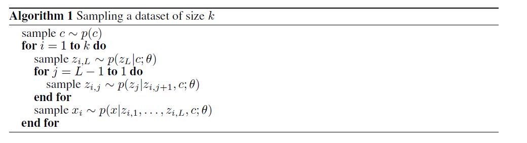
Generative Process :

Full Approximate posterior를 factorize하면…

• \[q\left(c, z_{1: L} \mid D ; \phi\right)=q(c \mid D ; \phi) \prod_{x \in D} q\left(z_{L} \mid x, c ; \phi\right) \prod_{i=1}^{L-1} q\left(z_{i} \mid z_{i+1}, x, c ; \phi\right)\]

ELBO를 세 가지 term으로 나눌 수 있음

• 1) Reconstruction term \(R_E\)
• 2) Context Divergence \(C_D\)
• 3) Latent Divergence \(L_D\)

\[\begin{aligned} &\mathcal{L}_{D}=R_{D}+C_{D}+L_{D} \text { with } \\ &R_{D}=\mathbb{E}_{q(c \mid D ; \phi)} \sum_{x \in D} \mathbb{E}_{q\left(z_{1: L} \mid c, x ; \phi\right)} \log p\left(x \mid z_{1: L}, c ; \theta\right) \\ &C_{D}=D_{K L}(q(c \mid D ; \phi) \| p(c)) \\ &L_{D}=\mathbb{E}_{q\left(c, z_{1: L} \mid D ; \phi\right)}\left[\sum_{x \in D} D_{K L}\left(q\left(z_{L} \mid c, x ; \phi\right) \| p\left(z_{L} \mid c ; \theta\right)\right)\right. \left. +\sum_{i=1}^{L-1} D_{K L}\left(q\left(z_{i} \mid z_{i+1}, c, x ; \phi\right) \| p\left(z_{i} \mid z_{i+1}, c ; \theta\right)\right)\right] \end{aligned}\]

Maximize the ELBO over 모든 datasets!

3-4. Statistic Network

(standard) inference network + \(\alpha\) … “Statistic Network” \(q(c \mid D;\phi)\)

FFNN에는 3가지 main element

• 1) 인코더 \(E\) : takes individual datapoint \(x_i\) to a vector \(e_i = E(x_i)\)
• 2) exchangeable instance pooling layer that collapses matrix \((e_1,...,e_k)\) to single pre-static vector \(v\)
• 3) final post-pooling network , that takes \(v\) to parameterization of diagonal Gaussian