(paper 82) Self-supervised learning of Split Invariant Equivariant representations

SSL of Split Invariant Equivariant representations

Contents

1. Abstract
2. Introduction
   1. 3DIEBench
   2. Hypernetwork based predictor
3. Related Works
   1. Invariant SSL
   2. Introducing Equivariance in Invariant SSL
   3. Equivariant Representation Learning
4. 3DIEBench : A new benchmark for invariant-equivariant SSL
5. Creating a general predictor
   1. Background and Notation
   2. SIE

0. Abstract

Towards learning INVARIANT or EQUIVARIANT representations with SSL

Evaluation

• Invariant methods : on LARGE scale datasets

• Equivariant methods : in SMALLER, more controlled, settings.

Bridging the gap between the two

\(\rightarrow\) to learn more diverse representations suitable for a wide range of tasks.

New dataset : 3DIEBench

• consisting of renderings from 3D models over 55 classes
• more than 2.5 million images
• full control on the transformations applied to the objects.

Predictor architecture

• based on hypernetworks to learn EQUIVARIANT representations with no possible collapse to INVARIANCE.

SIE (Split Invariant Equivariant) : combines the hypernetwork based predictor,

with representations split in 2 parts

• (1) invariant
• (2) equivariant

1. Introduction

SSL of image representations … catch up SL baselines

Most of the works : Joint-embedding framework

= 2 augmented views from a source image.

These INVARIANCE based approaches have been very successful for classification,

when using augmentations that preserve the semantic information of the image.

\(\rightarrow\) BUT…this removal of information may be problematic for downstream tasks.

• ex) color-jitter removes color information \(\rightarrow\) Bad for flower classification (Lee et al., 2021a).

Thus, motivates the goal of introducing “Equivariance” to representations

• to learn more general representations for more varied downstream tasks.

Previous ways ?

by keeping information about the augmentations

• ex) use subsets of augmentations to construct partially invariant representations

• ex) predicting rotations

• ex) preserving augmentation strengths in the representations

• ex) predicting all of the augmentation parameters

Common : do not give a way to transform the representations directly even if the information is present in them

\(\rightarrow\) cannot be considered as EQUIVARIANT.

Learning equivariant representations :

\(\rightarrow\) requires being able to predict a representation from another in LATENT SPACE,

• can be done by a simple prediction head

  ( ex. reconstruction task )

(1) Parameter prediction based methods

have been done on ImageNet

• no clear equivariant task and where augmentations happen in pixel space with no loss of information.

(2) Equivariance based methods

have been used on simpler synthetic datasets

• where we can evaluate equivariance
• but where it is hard to evaluate other CV tasks ( ex. classification )

To bridge the gap between those two

• (a) Introduce NEW datsaset, 3DIEBench
• (b) Introduce a hypernetwork based predictor

(1) 3DIEBench

• renderings of over fifty-thousand 3D objects

• can study both ..

  • Equivariance related task (3D rotation prediction)
  • Invariant related task (image classification).

• allows us to measure more precisely how invariant classical SSL are

• Shows limitations of existing equivariant approaches ,

  where predictors often collapse to the identity \(\rightarrow\) leading to invariant representations.

(2) Hypernetwork based predictor

• avoids a collapse to the identity by design
• show how it can outperform existing predictor architectures.

Also show that by “SEPARATING” the representations in (a) equivariant and (b) invariant parts,

\(\rightarrow\) can significantly improve performance on equivariance related tasks!!

Also analyze qualitatively the learned split invariant-equivariant representations

\(\rightarrow\) see that all invariant information is NOT DISCARDED from the equivariant part

& and that the predictor offers a meaningful way to steer the latent space.

2. Related Works

(1) Invariant SSL

Two main families of methods

a) CL

• mostly rely on the InfoNCE

• clustering variant of CL

  ( between cluster centroids instead of samples )

b) Non CL

• bringing together embeddings of positives, similar to CL

• Key difference ( with CL ) ??

  \(\rightarrow\) lies in how those methods prevent a representational collapse

  • (CL) pushes away negative
  • (Non CL) the criterion considers the embeddings as a whole & encourages information content maximization
    • ex) by regularizing the empirical covariance matrix of the embeddings.

CL & Non CL : They have been shown to lead to very similar representations

(2) Introducing Equivariance in Invariant SSL

( Invariant SSL : focus on learning representations that are invariant to augmentations )

\(\leftrightarrow\) Representations where information about certain transformations is preserved.

• ex) predicting the augmentation parameters
• ex) introducing other transformations such as image rotations
• ex) preserving the augmentations’ strength in the representations

\(\rightarrow\) these approaches* CAN NOT be characterized as equivariant* ,

since they offer no meaningful way to apply transformations in LATENT SPACE.

(3) Equivariant Representation Learning

Autoencoders

• transforming autoencoders
• Homeomorphic VAEs
• EquiMod (Devillers & Lefort, 2022) or SEN (Park et al., 2022)
  • included a predictor that enables the steering of representations in latent space, without requiring reconstruction.
  • Forms the basis for our comparisons.

(Marchetti et al., 2022)

• representations are split in (1) class and (2) pose

  ( i.e. invariant and equivariant )

• assumes a simple EQUIVARIANT latent space
  • the group action is the same as in the underlying data, e.g. 3 dimensions to represent pose.
  • assumes prior knowledge on the group of transformations
• This paper : aim at deriving a more general predictor architecture with no such priors

3. 3DIEBench: A new benchmark for invariant-equivariant SSL

a) Problems with previous datasets

Datasets to evaluate …

• Equivariance : due to the need to control HOW TRANSFORMATIONS ARE APPLIED

• Invariance : limited in the sense that position and shape of the objects in these dataset can not be parameterized by controllable transformations

  ( = only pixel-level transformations can be applied )

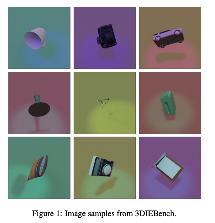
b) Dataset Intro

Introduce a new dataset, 3D Invariant Equivariant Benchmark (3DIEBench)

• Bridge the gap between the two
  • Not trivial for an INVARIANT task ( Image Classification )
  • Still have control on the parameter of the scene and the objects within it to learn meaningful EQUIVARIANT representations.
• Use renderings of 3D objects from the subset of ShapeNetCore (Chang et al., 2015) originating from 3d Warehouse (Trimble Inc).
• # of datasets : total 52472 objects spread across 55 classes.

c) Dataset Details

• Adjust various factors of variations

  ( ex. object rotation, the lighting color, or the floor color )

• Focus on learning representations that are …

  • EQUIVARIANT w.r.t object ROTATIONS of arbitrary strength

• constrain the range of rotations to Euler angles between \(-\frac{\pi}{2}\) ~ \(\frac{\pi}{2}\)

  • arbitrary rotations ?? NO! Make the task close to impossible

• For each object, generate 50 random values for the factors of variation

  \(\rightarrow\) total of around 2.5 million images.

4. Creating a general predictor

(1) Background & Notation

a) Group actions

• set \(G\) with a binary operation ·: \(G \times G \rightarrow G\),
  • exists an identity element \(e \in G\)
  • every element \(g \in G\) has an inverse \(g^{-1}\)
• focus is on 3D rotation ….. \(S O(3)\),
  • use quaternions to represent them, i.e. \(S p(1)\),

• function \(\alpha\) : \(G \times S \rightarrow S\)

  • such that \(\alpha(e, s)=s\)

  • \(\alpha(g, \alpha(h, x))=\) \(\alpha(g h, x)\).

  • If \(\alpha\) is linear & acts on a vector space \(V\) such as \(\mathbb{R}^n\),

    \(\rightarrow\) called a group representation.

• Define a group representation as the map \(\rho: G \rightarrow G L(V)\)
  • such that \(\rho(g)=\alpha(g, \cdot)\).
• ex) Input image \(x\) & Augmented view \(x^{\prime}\) :
  • defined as \(x^{\prime}=\rho(g) \cdot x\), where \(g\) describes the augmentation parameters.

b) Invariant SSL

Dataset \(\mathcal{D}\) with datum \(d \in \mathbb{R}^{c \times h \times w}\)

Procedure

• (1) Generate 2 views \(x\) and \(x^{\prime}\)

• (2) Fed through an encoder \(f_\theta\)

  • \(y=f_\theta(x)\) and \(y^{\prime}=f_\theta\left(x^{\prime}\right)\).

• (3) Fed through a projection head \(h_\phi\)

  • \(z=h_\phi(y)\) and \(z^{\prime}=h_\phi\left(y^{\prime}\right)\).

• (4) Goal : Make \(\left(z, z^{\prime}\right)\) identical to learn embeddings

  • that are invariant to the applied augmentations
  • extract meaningful information from the original images.

Consider the DA strategy as a group representation \(\rho_X\).

• \(x=\rho_X\left(g_1\right) \cdot d\).
• \(x^{\prime}=\rho_X\left(g_2\right) \cdot d\) .
  • \(x^{\prime}=\rho_X(g) \cdot d\) with \(g=g_1^{-1} \cdot g_2\).

Goal of Invariant SSL :

\(\rightarrow\) \(\forall x \in \mathcal{D} \forall g \in G, h_\phi\left(f_\theta(x)\right)=h_\phi\left(f_\theta\left(\rho_X(g) \cdot x\right)\right)\).

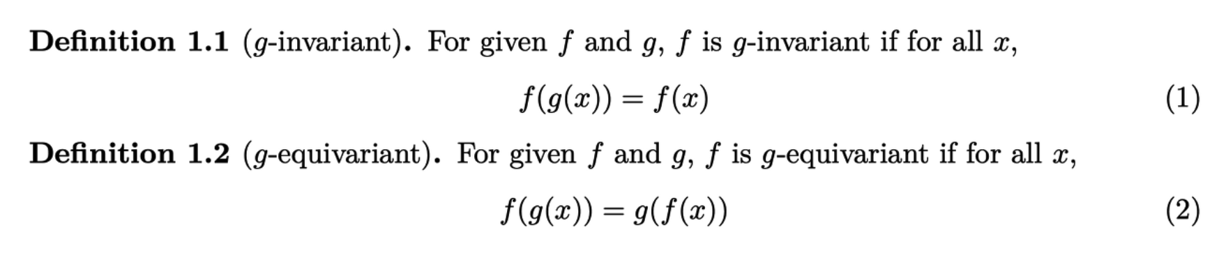
c) Equivariant Representations

Given a group \(G\) with representations \(\rho_X\) and \(\rho_Y\), ….

Function \(f: X \rightarrow Y\) is equivariant w.r.t \(G\) if \(\forall x \in X, \forall g \in G\) we have

• \(f\left(\rho_X(g) \cdot x\right)=\rho_Y(g) \cdot f(x)\).

Invariance is just a special case! where \(\rho_Y(g)=I d\).

\(\rightarrow\) Common failure mode of existing equivariant approaches.

Prior works : focused on forcing equivariance by the architecture of \(f\)

This paper : focus in a setting where this is not possible, and where we do not even know \(\rho_X\).

\(\rightarrow\) Goal : Learn both \(f\) and \(\rho_Y\) to obtain representations that are as equivariant as possible to the original transformation.

(2) SIE

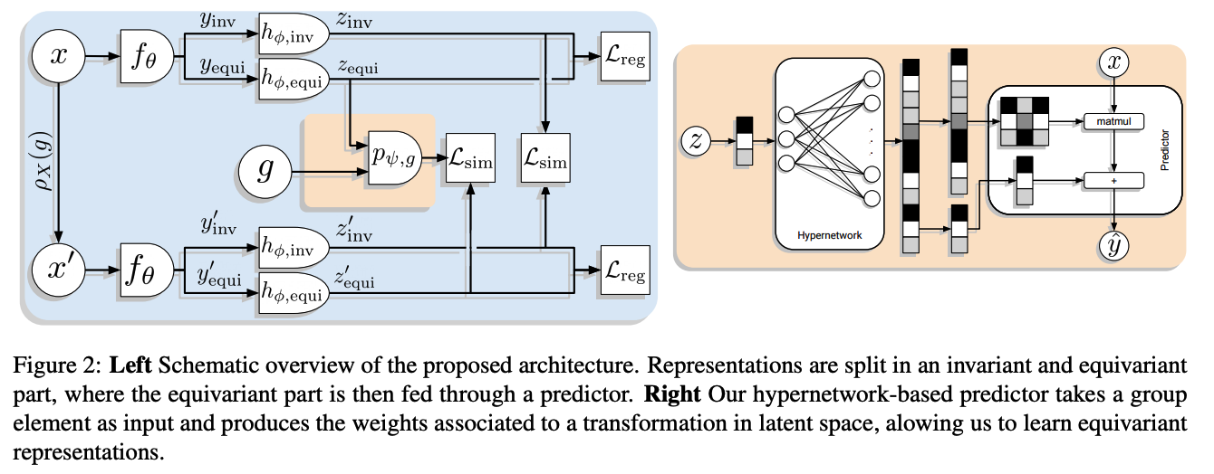
Introduce a split in 2 of the representations ( before the projection head )

• \(y_{\text {inv }}\) : contains information that is preserved by the transformation ( = Invariant information )

• \(y_{\text {equi }}\) : contains information that was changed by the transformation ( = Equivariant information )

• \(y\) = 512-dim …. 256 / 256-dim split

\(\rightarrow\) call Split Invariant Equivariant (SIE).

Fed to separate projection heads \(h_{\phi \text {,inv }}\) and \(h_{\phi, \text { equi }}\)

• no information exchange after the split.
• embeddings \(z_{\mathrm{inv}}\) and \(z_{\text {equi }}\).

Goal :

• Invariant embeddings \(z_{\text {inv }}\) and \(z_{\text {inv }}^{\prime}\) to be identical
• Equivariant embeddings \(z_{\text {equi }}\) and \(z_{\text {equi }}^{\prime}\) to be only identical after the predictor \(p_{\psi, g}\),

Predictor \(p_{\psi, g}\) ( figure 2 )

• learnable \(\rho_Y(g)\) described previously

Loss function : based on VICReg

• To adapt its invariance criterion, define our similarity criterion \(\mathcal{L}_{\text {sim }}\) as

  • \(\mathcal{L}_{\text {sim }}(u, v)=\mid \mid u-v \mid \mid_2^2\).

  • to match both our invariant & equivariant pairs.

• To avoid a collapse of the representations, we use the original & and covariance criterion to define our regularisation criterion \(\mathcal{L}_{\text {reg }}\) as

  • \(\begin{aligned} \mathcal{L}_{\mathrm{reg}}(Z) & =\lambda_C C(Z)+\lambda_V V(Z), \quad \text { with } \\ C(Z) & =\frac{1}{d} \sum_{i \neq j} \operatorname{Cov}(Z)_{i, j}^2 \quad \text { and } \\ V(Z) & =\frac{1}{d} \sum_{j=1}^d \max \left(0,1-\sqrt{\operatorname{Var}\left(Z_{\cdot, j}\right)}\right) \end{aligned}\).
    • variance criterion \(V\) : Ensure that all dimensions are used in the embeddings
    • covariance criterion \(C\) : Decorrelate the dimensions to spread out informations

Final Loss function

\(\begin{aligned} \mathcal{L}_{\mathrm{SIE}}\left(Z, Z^{\prime}\right)= & \mathcal{L}_{\text {reg }}\left(Z^{\prime}\right)+\mathcal{L}_{\text {reg }}(Z)+\lambda_V V\left(p_{\psi, g_i}\left(Z_{i, \text { equi }}\right)\right)+ \\ & \lambda_{\text {inv }} \frac{1}{N} \sum_{i=1}^N \mathcal{L}_{\text {sim }}\left(Z_{i, \text { inv }}, Z_{i, \text { inv }}^{\prime}\right)+ \\ & \lambda_{\text {equi }} \frac{1}{N} \sum_{i=1}^N \mathcal{L}_{\text {sim }}\left(p_{\psi, g_i}\left(Z_{i, \text { equi }}\right), Z_{i, \text { equi }}^{\prime}\right) . \end{aligned}\).