(paper 81) TSMixer; An all-MLP Architecture for TS Forecasting

TSMixer: An all-MLP Architecture for TS Forecasting

Contents

1. Abstract
2. Introduction
3. Related Works
4. Linear Models for TS Forecasting
   1. Theoretical Insights
   2. Differences from DL
5. TSMixer Architecture
   1. TSMixer for MTS Forecasting
   2. Extended TSMixer for TS Forecasting with Auxiliary Information
      1. align
      2. mixing
6. Experiments
   1. MTS LTSF
   2. M5

0. Abstract

DL basd on RNN/Transformer ??

NO!! Simple univariate linear models can outperform such DL models

This paper

• investigate the capabilities of linear models for TS forecasting
• present Time-Series Mixer (TSMixer)

TSMixer

• a novel architecture designed by stacking MLPs

• based on mixing operations along both the time & feature dimensions

• simple-to-implement

Results

• SOTA

• Underline the importance of efficiently utilizing cross-variate & auxiliary information
• various analyses

1. Introduction

The forecastability of TS often originates from 3 major aspects:

• (1) Persistent temporal patterns
  • trend & seaonal patterns
• (2) Cross-variate information
  • correlations between different variables
• (3) Auxiliary Features
  • comprising static features and future information

ARIMA (Box et al., 1970)

• for UTS forecasting
• only temporal information is available

DL ( Transformer-based models )

• capture both complex temporal patterns & cross-variate dependencies

• MTS model : should be more effective than UTS model

  • due to their ability to leverage cross-variate information.

  ( \(\leftrightarrow\) Simple Linear model ( Linear / DLinear / NLinear ) by Zeng et al. (2023) )

  • MTS model seem to suffer from overfitting

    ( especially when the target TS is not correlated with other covariates )

2 essential questions

Analyzing the effectiveness of temporal linear models.

Gradually increase the capacity of linear models by

1. stacking temporal linear models with non-linearities (TMix-Only)
2. introducing cross-variate feed-forward layers (TSMixer)

TSMixer

• time-mixing & feature-mixing

  • alternatively applies MLPs across time and feature dimensions

• residual designs

  • ensure that TSMixer retains the capacity of temporal linear models,

    while still being able to exploit cross-variate information.

Experiment 1

Datasets : long-term forecasting datasets (Wu et al., 2021)

( where UTS models » MTS models )

Ablation study

• effectiveness of stacking temporal linear models

• cross-variate information is less beneficial on these popular datasets

  ( = explaining the superior performance of UTS models. )

• Even so, TSMixer is on par with SOTA UTS models

Experiment 2

( to demonstrate the benefit of MTS models )

Datasets : challenging M5 benchmark

• a large-scale retail dataset used in the M-competition
• contains crucial cross-variate interactions
  • such as sell prices

Experiments

• cross-variate information indeed brings significant improvement!

  ( + TSMixer can effectively leverage this information )

Propose a principle design to extend TSMixer…

\(\rightarrow\) to handle auxiliary information

• ex) static features & future time-varying features.

• Details : aligns the different types of features into the same shape

  & applied mixer layers on the concatenated features to leverage the interactions between them.

Applications

outperforms models that are popular in industrial applications

• ex) DeepAR (Salinas et al. 2020, Amazon SageMaker) & TFT (Lim et al. 2021, Google Cloud Vertex)

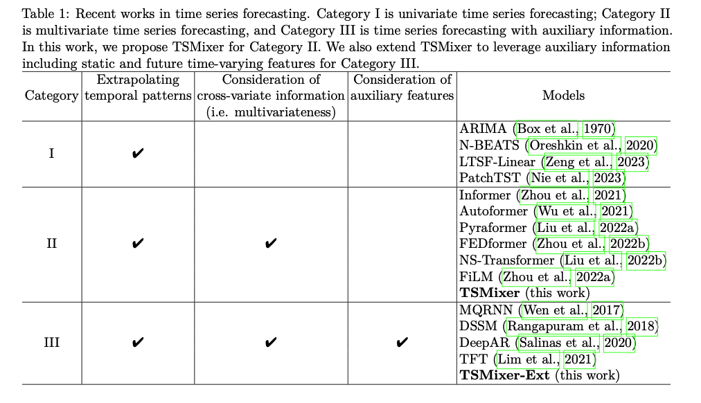
2. Related Works

Table 1 : split into three categories

• (1) UTS forecasting
• (2) MTS forecasting
• (3) MTS forecasting with auxiliary information.

MTS forecasting

• Key Idea : modeling the complex relationships between covariates should improve the forecasting performance
• Example : Transformer-based models
  • superior performance in modeling long and complex sequential data
  • ex) Informer (Zhou et al., 2021) and Autoformer (Wu et al., 2021)
    • tackle the efficiency bottleneck
  • ex) FEDformer (Zhou et al., 2022b) and FiLM (Zhou et al., 2022a)
    • decompose the sequences using FFT
  • ex) ETC
    • improving specific challenges, such as non-stationarity (Kim et al., 2022; Liu et al., 2022b).

UTS works better??

• Linear / DLinear /NLinear ( Zeng et al. (2023) )
  • show the counter-intuitive result that a simple UTS linear model
• PatchTST ( Nie et al. (2023) )
  • advocate against modeling the cross-variate information
  • propose a univariate patch Transformer for MTS forecasting

This paper :

• UTS » MTS ?? NO! Dataset Bias!

Use along with Auxiliary information

• static features (e.g. location)
• future time-varying features (e.g. promotion in coming weeks),

Algorithms example )

• ex) state-space models (Rangapuram et al., 2018; Alaa & van der Schaar, 2019; Gu et al., 2022)
• ex) RNN variants ( Wen et al. (2017); Salinas et al. (2020) )
• ex) Attention models ( Lim et al. (2021) )

\(\rightarrow\) Real-world time-series datasets are more aligned with this setting!

\(\rightarrow\) \(\therefore\) achieved great success in industry

• DeepAR (Salinas et al., 2020) of AWS SageMaker
• TFT (Lim et al., 2021) of Google Cloud Vertex).

\(\leftrightarrow\) Drawback : complexity

Motivations for TSMixer

stem from analyzing the performance of linear models for TS forecasting.

3. Linear Models for TS Forecasting

(1) Theoretical insights on the capacity of linear models

• have been overlooked due to its simplicity

(2) Compare linear models with other architectures

• show that linear models have a characteristic not present in RNNs and Transformers

  ( = Linear models have the appropriate representation capacity to learn the time dependency for a UTS )

Notation

\(\boldsymbol{X} \in \mathbb{R}^{L \times C_x}\) : input

\(\boldsymbol{Y} \in \mathbb{R}^{T \times C_y}\) : target

Focus on the case where \(\left(C_y \leq C_x\right)\)

Linear model params : \(\boldsymbol{A} \in \mathbb{R}^{T \times L}, \boldsymbol{b} \in \mathbb{R}^{T \times 1}\)

• \(\hat{\boldsymbol{Y}}=\boldsymbol{A} \boldsymbol{X} \oplus \boldsymbol{b} \in \mathbb{R}^{T \times C_x}\).
  • \(\oplus\) : column-wise addition

(1) Theoretical insights

Most impactful real-world applications have either ..

• (1) smoothness
• (2) periodicity

Assumption 1) Time series is periodic (Holt, 2004; Zhang \& Qi, 2005).

(A) arbitrary periodic function \(x(t)=x(t-P)\), where \(P<L\) is the period.

perfect solution :

• \(\boldsymbol{A}_{i j}=\left\{\begin{array}{ll} 1, & \text { if } j=L-P+(i \bmod P) \\ 0, & \text { otherwise } \end{array}, \boldsymbol{b}_i=0 .\right.\).

(B) affine-transformed periodic sequences, \(x(t)=a \cdot x(t-P)+c\), where \(a, c \in \mathbb{R}\) are constants

perfect solution :

• \(\boldsymbol{A}_{i j}=\left\{\begin{array}{ll} a, & \text { if } j=L-P+(i \bmod P) \\ 0, & \text { otherwise } \end{array}, \boldsymbol{b}_i=c .\right.\).

Assumption 2) Time series can be decomposed into a periodic sequence and a sequence with smooth trend

• proof in Appendix A

(2) Differences from DL

Deeper insights into why previous DL models tend to overfit the data

• Linear models = “time-step-dependent”
  • weights of the mapping are fixed for each time step
• Recurrent / Attention models = “data-dependent”
  • weights over the input sequence are outputs of a “data-dependent” function

Time-step-dependent models vs. Data-dependent models

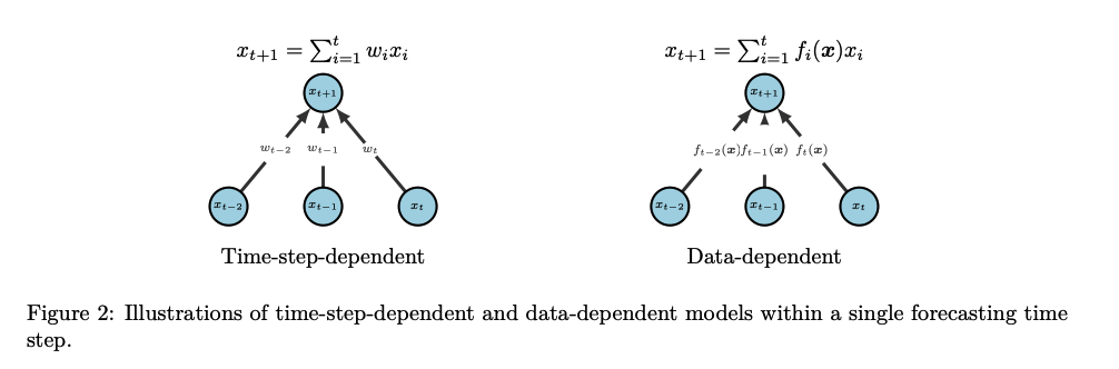
Time-step-dependent linear modes

• simple
• highly effective in modeling temporal patterns

Data-dependent models

• high representational capacity

  ( = achieving time-step independence is challenging )

• usually overfit on the data

  ( = instead of solely considering the positions )

4. TSMixer Architecture

Propose a natural enhancement by stacking linear models with non-linearities

Use common DL techniques

• normalization
• residual connections

\(\rightarrow\) However, this architecture DOES NOT take cross-variate information into account.

For cross-variate information…

\(\rightarrow\) we propose the application of MLPs in

• the time-domain
• the feature-domain

in an alternating manner.

Time-domain MLPs

• shared across all of the features

Feature-domain MLPs

• shared across all of the time steps.

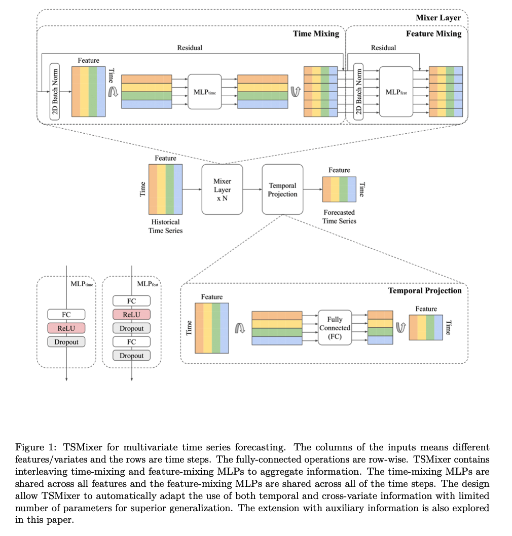
Time-Series Mixer (TSMixer)

Interleaving design between these 2 operations

• efficiently utilizes both TEMPORAL dependencies & CROSS-VARIATE information

  ( while limiting computational complexity and model size )

• allows to use a long lookback window

  • parameter growth in only \(O(L+C)\), not \(O(LC)\) if FC-MLPs were used

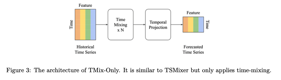
TMix-Only : also consider a simplified variant of TSMixer

• only employs time-mixing
• consists of a residual MLP shared across each variate

Extension of TSMixer with auxiliary information

(1) TSMixer for MTS Forecasting

TSMixer applies MLPs alternatively in (1) time and (2) feature domains.

Components

• Time-mixing MLP:

  • for temporal patterns
  • FC layer & activation function & dropout
  • transpose the input
    • to apply the FC layers along the time domain ( shared by features )
  • single-layer MLP ( already proves to be a strong model )

• Feature-mixing MLP:

  • shared by time steps
  • leverage covariate information
  • two-layer MLPs

• Temporal Projection:

  • FC layer applied on time domain

  • not only learn the temporal patterns,

    but also map the TS from input length \(L\) to forecast length \(T\)

• Residual Connections:

  • between each (1) time-mixing and (2) feature-mixing MLP
  • learn deeper architectures more efficiently
  • effectively ignore unnecessary time-mixing and feature-mixing operations.

• Normalization:

  • preference between BN and LN is task-dependent
    • ( Nie et al. (2023) ) advantages of BN on common TS
    • apply 2D normalization on both time & feature dimensions

Architecture of TSMixer is relatively simple to implement.

(2) Extended TSMixer for TS Forecasting with Auxiliary Information

Real-world scenarios : access to ..

• (1) static features : \(\boldsymbol{S} \in \mathbb{R}^{1 \times C_s}\)
• (2) future time-varying features : \(\boldsymbol{Z} \in \mathbb{R}^{T \times C_z}\)

\(\rightarrow\) extended to multiple TS, represented by \(\boldsymbol{X}^{(i)}{ }_{i=1}^N\),

• \(N\) : number of TS

Long-term forecasting

• ( In general ) Only consider the historical features & targets on all variables

  (i.e. \(\left.C_x=C_y>1, C_s=C_z=0\right)\).

• ( In this paper ) Also consider the case where auxiliary information is available

  (i.e. \(C_s>0, C_z>0\) ).

To leverage the different types of features…

\(\rightarrow\) Propose a principle design that naturally leverages the feature mixing to capture the interaction between them.

• (1) Design the align stage
  • to project the feature with different shapes into the same shape.
• (2) Concatenate the features
  • apply feature mixing on them.

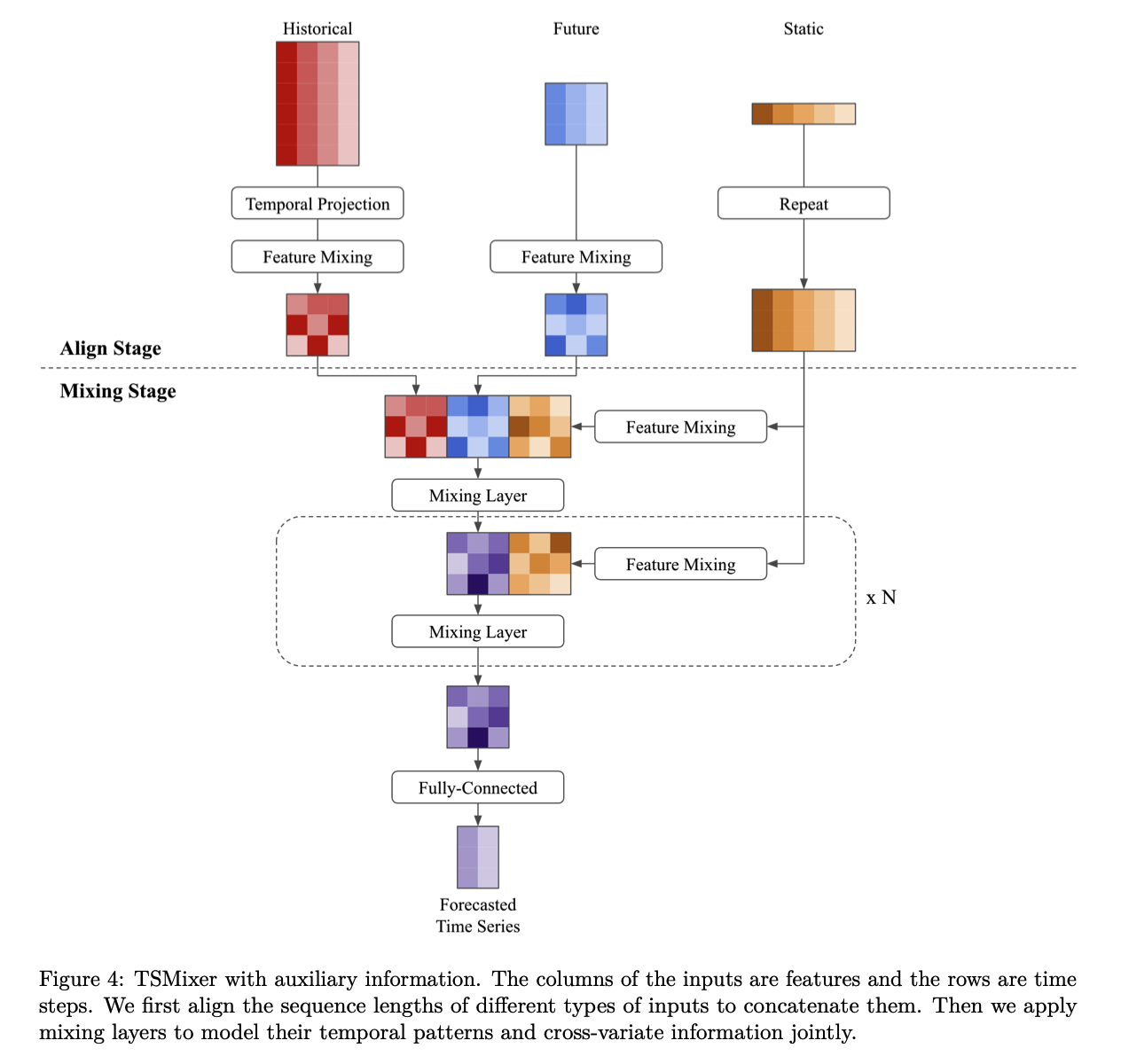
Architecture comprises 2parts:

• (1) align
• (2) mixing.

a) Align

aligns historical features \(\left(\mathbb{R}^{L \times C_x}\right)\) and future features ( \(\left.\mathbb{R}^{T \times C_z}\right)\) into the same shape \(\left(\mathbb{R}^{L \times C_h}\right)\)

• [Historical input] apply temporal projection & feature-mixing layer
• [Future input] apply feature-mixing layer
• [Static input] repeat to transform their shape from \(\mathbb{R}^{1 \times C_s}\) to \(\mathbb{R}^{T \times C_s}\)

b) Mixing

Mixing layer

• time-mixing & feature-mixing operations

• leverages temporal patterns and cross-variate information from all features collectively.

FC layer

• to generate outputs for each time step.
• slightly modify mixing layers to better handle M5 dataset ( described in Appendix \(B\) )

5. Experiments

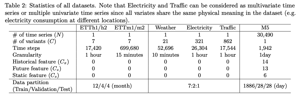
Datasets

• 7 popular MTS long-term forecasting benchmarks
  • w/o auxiliary information
• Large-scale real-world retail dataset, M5
  • w auxiliary information
  • containing 30,490 TS with static features & time-varying features
  • more challenging

[ MTS forecasting benchmarks ] Settings

• input length \(L = 512\)
• prediction lengths of \(T = \{96, 192, 336, 720\}\)
• Adam optimization
• Loss : MSE
• Metric : MSE & MAE
• Apply reversible instance normalization (Kim et al., 2022) to ensure a fair comparison with the state-of-the-art PatchTST (Nie et al., 2023).

[ M5 dataset ] Settings

• data processing from Alexandrov et al. (2020).
• input length \(L=35\)
• prediction length of \(T = 28\)
• Loss : log-likelihood of negative binomial distribution
• follow the competition’s protocol to aggregate the predictions at different levels
• Metric : WRMSSE ( Weighted Root Mmean Squared Scaled Error )

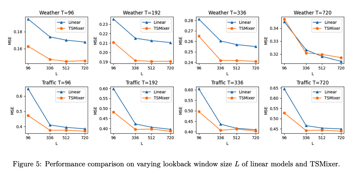
(1) MTS LTSF

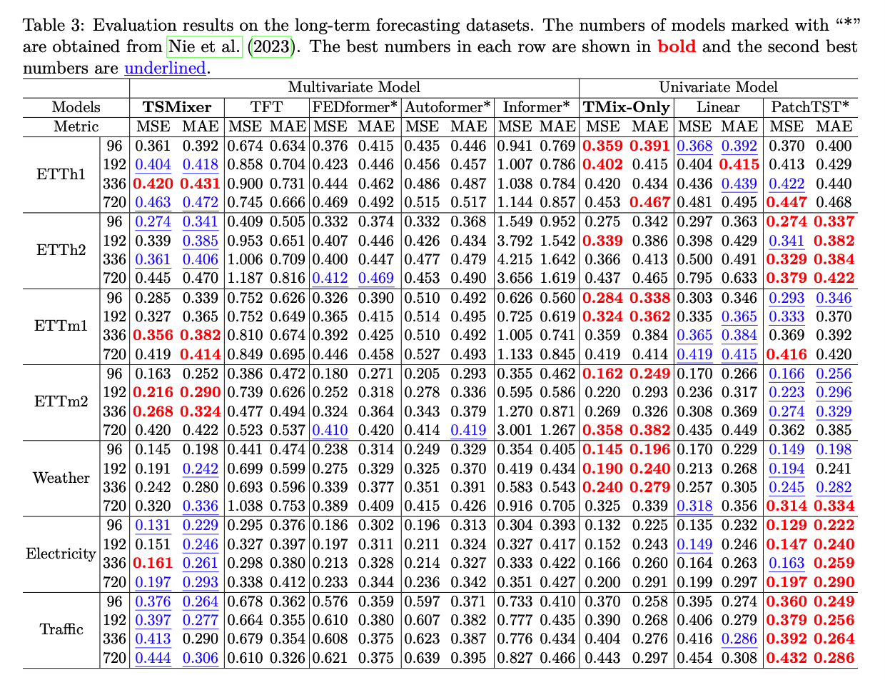
Effects of \(L\)

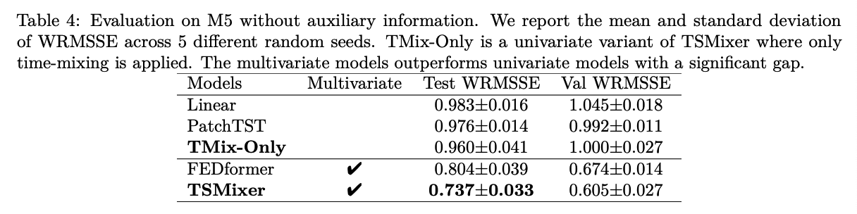
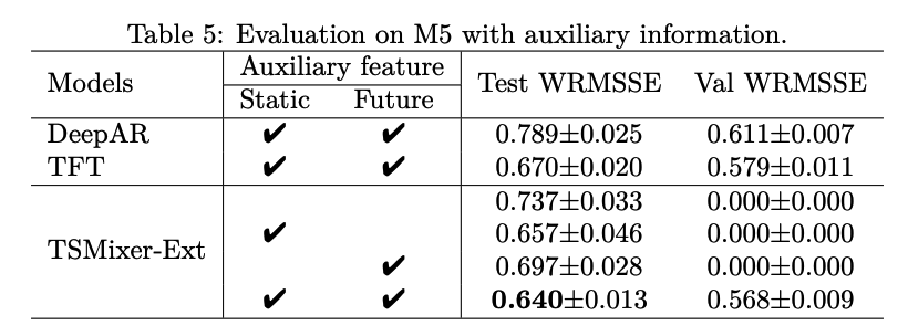
(2) M5

to explore the model’s ability to leverage

• (1) cross-variate information
• (2) auxiliary features

Forecast with HISTORICAL features only

Forecast with AUXILIARY information

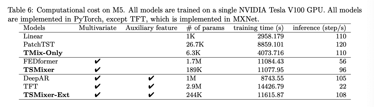
Computational Cost