
Vision Transformer for Small-Size Datasets
Contents
- Abstract
- Introduction
- 2 problems
- 2 proposals
- Proposed Method
- Preliminary
- Shifted Patch Tokenization (SPT)
- Locality Self-Attention (LSA)
- Experiments
0. Abstract
High performance of the ViT results from …
$\rightarrow$ pre-trainingusing a “large-size dataset” ( such as JFT-300M )
Why large datsaet?
$\rightarrow$ due to “low locality inductive bias”
Proposes ..
- (1) Shifted Patch Tokenization (SPT)
- (2) Locality Self-Attention (LSA)
effectively solve the lack of locality inductive bias
& enable it to learn from scratch even on small-size datasets
& generic and effective add-on modules that are easily applicable to various ViTs.
 .
.
1. Introduction
(1) 2 problems
2 problems that decrease locality inductive bias & limit the performance of ViT
1) Poor “tokenization”
-
divides an image into non-overlapping patches of equal size
$\rightarrow$ non-overlapping : allow visual tokens to have a relatively small receptive field than overlapping patches
$\rightarrow$ cause ViT to tokenize with too few pixels
$\rightarrow$ [PROBLEM 1] spatial relationship with adjacent pixels is not sufficiently embedded in each visual token
-
linearly projects each patch to a visual token.
( same linear projection is applied to each patch )
$\rightarrow$ permutation invariant property
- enables a good embedding of relations between patches
2) Poor “attention mechanism”
feature dim of image data : greater than that of natural language
$\rightarrow$ number of embedded tokens is inevitably large
$\rightarrow$ distn of attention scores of tokens becomes smooth
( = cannot attend locally to important visual tokens )
Problem 1) & 2)
$\rightarrow$ cause highly redundant attentions that cannot focus on a target class
$\rightarrow$ redundant attention : concentrate on background, not the shape of the target class!
(2) 2 Proposals
two solutions to effectively improve the locality inductive bias of ViT for learning small-size datasets from scratch
1) Shifted Patch Tokenization (SPT)
- to further utilize ”SPATIAL relations between neighboring pixels in the tokenization process
- idea from Temporal Shift Module (TSM)
- TSM : effective temporal modeling which shifts some temporal channels of features
- SPT : effective spatial modeling that tokenizes spatially shifted images together with the input image
- result : can give a wider receptive field to ViT than standard tokenization
2) Locality Self-Attention (LSA)
-
allows ViTs to “attend locally”
-
mitigates the smoothing phenomenon of attention score distn
- HOW?
- (1) by excluding self-tokens
- (2) by applying learnable temperature to the softmax function
-
induces attention to work locally,
by forcing each token to focus more on tokens with large relation to itself
Both SPT and LSA : can be easily applied to various ViTs
2. Proposed Method
describes 2 key ideas for increasing the locality inductive bias of ViTs
$\rightarrow$ SPT & LSA
 .
.
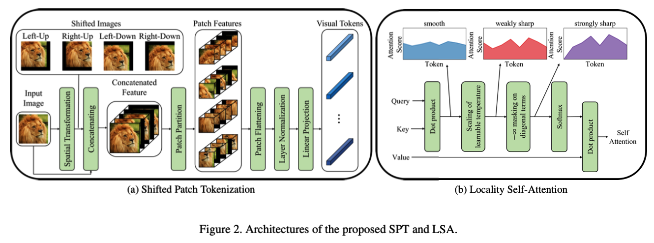
Shifted Patch Tokenization (SPT)
-
step 1) spatially shifts an input image in several directions & concatenates them with the input image
-
step 2) patch partitioning
- step 3) embedding into visual tokens
- 3-1) patch flattening
- 3-2) layer normalization
- 3-3) linear projection
-
Result )
-
can embed more spatial information into visual tokens
-
increase the locality inductive bias of ViTs
-
Locality Self-Attention (LSA)
- sharpens the distn of attention scores by learning the temperature parameters
- self-token relation is removed by applying “diagonal masking”
- suppresses thed iagonal components of the similarity matrix computed by Query and Key
- increases the atten-ion scores between different tokens
- Result) increases the locality inductive bias by making ViT’s attention locally focused.
(1) Preliminary
Reviews the tokenization and self-attention
Notation :
- $\mathbf{x} \in \mathbb{R}^{H \times W \times C}$: input image
Process
-
step 1) divides the input image into non-overlapping patches & flatten the patches to obtain a sequence of vectors
- $\mathcal{P}(\mathbf{x})=\left[\mathbf{x}_p^1 ; \mathbf{x}_p^2 ; \ldots ; \mathbf{x}_p^N\right]$
- $\mathbf{x}_p^i \in \mathbb{R}^{P^2 \cdot C}$ : the $i$-th flattened vector
- $P$ : patch size ( small H & small W )
- $N=H W / P^2$ : nubmer of patches
-
step 2) obtain patch embeddings
- by linear projection
- tokenization = step 1) + step 2)
- $\mathcal{T}(\mathbf{x})=\mathcal{P}(\mathbf{x}) \boldsymbol{E}_t$.
- $\boldsymbol{E}_t \in \mathbb{R}^{\left(P^2 \cdot C\right) \times d}$ : learnable linear projection for tokens
- $d$ : hidden dimension of transformer encoder
receptive fields of visual tokens in ViT are determined by tokenization
-
receptive field size of visual tokens : $r_{\text {token }}=r_{\text {trans }} \cdot j+(k-j)$
-
receptive field is not adjusted in the transformer encoder, so $r_{\text {trans }}=1$.
$\rightarrow$ $r_{\text {token }}$ is the same as the kernel size ( = patch size of ViT )
-
step 3) self-attention mechanism
-
3-1) learnable linear projection to obtain Q,K,V
-
3-2) calculate similarity matrix : $\mathrm{R} \in$ $\mathbb{R}^{(N+1) \times(N+1)}$
$\mathrm{R}(\mathbf{x})=\mathbf{x} \boldsymbol{E}_q\left(\mathbf{x} \boldsymbol{E}_k\right)^{\top}$.
- dot product operation of Q & K
- diagonal components of $\mathrm{R}$ : self-token relations
- off-diagonal components of $\mathrm{R}$ : intertoken relations:
- $\boldsymbol{E}_q \in \mathbb{R}^{d \times d_q}, \boldsymbol{E}_k \in \mathbb{R}^{d \times d_k}$ : learnable linear projections for Q & K
-
3-3) $\mathrm{SA}(\mathbf{x})=\operatorname{softmax}\left(\mathrm{R} / \sqrt{d_k}\right) \mathbf{x} \boldsymbol{E}_v$.
-
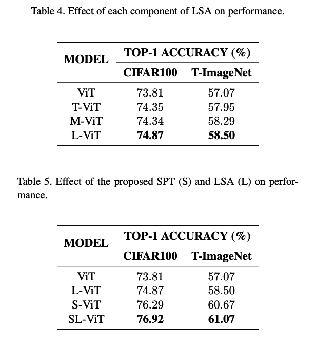
(2) Shifted Patch Tokenization (SPT)
applies the proposed SPT to …
- (1) the patch embedding layer
- (2) the pooling layer
step 1) input image is spatially shifted by 1/2 of the patch size in 4 diagonal directions
-
left-up, right-up, left-down, and right-down
-
$\mathcal{S}$ : shifting strategy
( various shifting strategies other than $\mathcal{S}$ are available )
step 2) shifted features are cropped to the same size as the input image & concatenated with the input
step 3) concatenated features are divided into non-overlapping patches & flattened
- like $\mathcal{P}(\mathbf{x})=\left[\mathbf{x}_p^1 ; \mathbf{x}_p^2 ; \ldots ; \mathbf{x}_p^N\right]$
step 4) visual tokens are obtained through layer normalization (LN) and linear projection
- $\mathrm{S}(\mathbf{x})=\operatorname{LN}\left(\mathcal{P}\left(\left[\mathbf{x} \mathbf{s}^1 \mathbf{s}^2 \ldots \mathbf{s}^{N_{\mathcal{S}}}\right]\right)\right) \boldsymbol{E}_{\mathcal{S}}$.
a) Patch Embedding Layer
how to use SPT as patch embedding?
$\rightarrow$ concatenate a class token to visual tokens & add positional embedding.
$\mathrm{S}{p e}(\mathbf{x})= \begin{cases}{\left[\mathbf{x}{c l s} ; \mathrm{S}(\mathbf{x})\right]+\boldsymbol{E}{p o s}} & \text { if } \mathbf{x}{c l s} \text { exist } \ \mathrm{S}(\mathbf{x})+\boldsymbol{E}_{p o s} & \text { otherwise }\end{cases}$.
b) Pooling Layer
if tokenization is used as a pooling layer…
$\rightarrow$ # of visual tokens can be reduced.
step 1) class tokens & visual tokens are separated
step 2) visual tokens are reshaped from 2D to 3D
- i.e., $\mathcal{R}: \mathbb{R}^{N \times d} \rightarrow$ $\mathbb{R}^{(H / P) \times(W / P) \times d}$.
step 3) New visual tokens ( with a reduced number of tokens ) are embedded
step 4) Linearly projected class token is connected with the embedded visual tokens
$\mathrm{S}{\text {pool }}(\mathbf{y})= \begin{cases}{\left[\mathbf{x}{c l s} \boldsymbol{E}{c l s} ; \mathrm{S}(\mathcal{R}(\mathbf{y}))\right]} & \text { if } \mathbf{x}{c l s} \text { exist } \ \mathrm{S}(\mathcal{R}(\mathbf{y})) & \text { otherwise }\end{cases}$.
(3) Locality Self-Attention (LSA)
Core of LSA :
- a) diagonal masking
- b) learnable temperature scaling
a) Diagonal Masking
$\mathrm{R}{i, j}^M(\mathbf{x})= \begin{cases}\mathrm{R}{i, j}(\mathbf{x}) & (i \neq j) \ -\infty & (i=j)\end{cases}$.
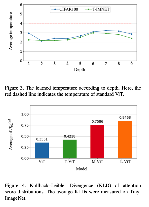
b) Learnable Temperature Scaling
$\mathrm{L}(\mathbf{x})=\operatorname{softmax}\left(\mathrm{R}^{\mathrm{M}}(\mathbf{x}) / \tau\right) \mathbf{x} \boldsymbol{E}_v$.
 .
.
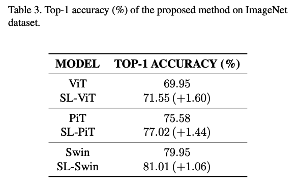
3. Experiments
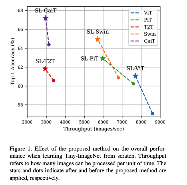
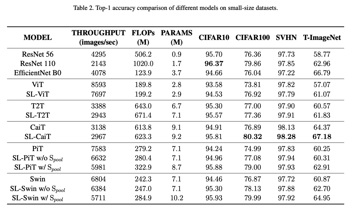
(1) Small-sized Datasets
 .
.
 .
.
(2) Ablation Studies
 .
.