
Adaptive Soft Contrastive Learning
Contents
-
Abstract
-
Introduction
-
Related Works
-
Adaptive Soft Contrastive Learning
- Soft CL
-
Adaptive Relabeling
- Distribution Sharpening
0. Abstract
Contrastive learning
- generally based on instance discrimination tasks
Problem : presuming all the samples are different
\(\rightarrow\) contradicts the natural grouping of similar samples in common visual datasets
Propose ASCL (Adaptive Soft Contrastive Learning)
-
adaptive method that introduces soft inter-sample relations
- original instance discrimination task \(\rightarrow\) multi-instance soft discrimination task
- adaptively introduces inter-sample relations
1. Introduction
focus on an inherent deficiency of contrastive learning, “class collision”
( = problem of false negatives )
\(\rightarrow\) Need to introduce meaningful inter-sample relations in contrastive learning.
ex 1) Debiased contrastive learning
- proposes a theoretical unbiased approximation of contrastive loss with the simplified hypothesis of the dataset distribution
- however, does not address the issue of real false negatives
ex 2) remove false negatives using progressive mechanism
- NNCLR : define extra positives for each specific view
- by ranking and extracting the top-K neighbors in the learned feature space.
- Co2 : introduces a consistency regularization
- enforcing relative distribution consistency of different positive views to all negatives
ex 3) Clustering-based approaches
-
also provide additional positives!
-
problems
- (1) assuming the entire cluster is positive early in the training is problematic
-
(2) clustering has an additional computational cost
- (3) all these methods rely on a manually set threshold or a predefined number of neighbors
ASCL
-
efficient and effective module for current contrastive learning frameworks
-
introduce inter-sample relations in an adaptive style
-
Similarity Distribution
-
use weakly augmented views to compute the relative similarity distribution
& obtain the sharpened soft label information.
-
based on the uncertainty of the similarity distribution, adaptively adjust the weights of the soft labels
-
-
Process
- (early stage) weights of the soft labels are low and the training of the model will be similar to the original contrastive learning
- (mature stage) soft labels become more concentrated
- the model will learn stronger inter-sample relations
Main Contributions
- propose a novel adaptive soft contrastive learning (ASCL) method
- smoothly alleviates the false negative & over-confidence in the instance discrimination
- reduces the gap between instance-based learning with cluster-based learning
- show that weak augmentation strategies help to stabilize the CL
- show that ASCL keeps a high learning speed in the initial epochs
2. Related Works
Introducing Inter-sample relations
how to introduce inter-sample relations into the original instance discrimination task.
ex) NNCLR :
-
builds on SimCLR by introducing a memory bank
-
searches for nearest neighbors to replace the original positive samples
ex) MeanShift :
- relies on the same idea but builds on BYOL.
ex) Co2
- an extra regularization term
- to ensure the relative consistency of both positive views with negative samples
ex) ReSSL
- validates that the consistency regularization term itself is enough to learn meaningful representations
3. Adaptive Soft Contrastive Learning
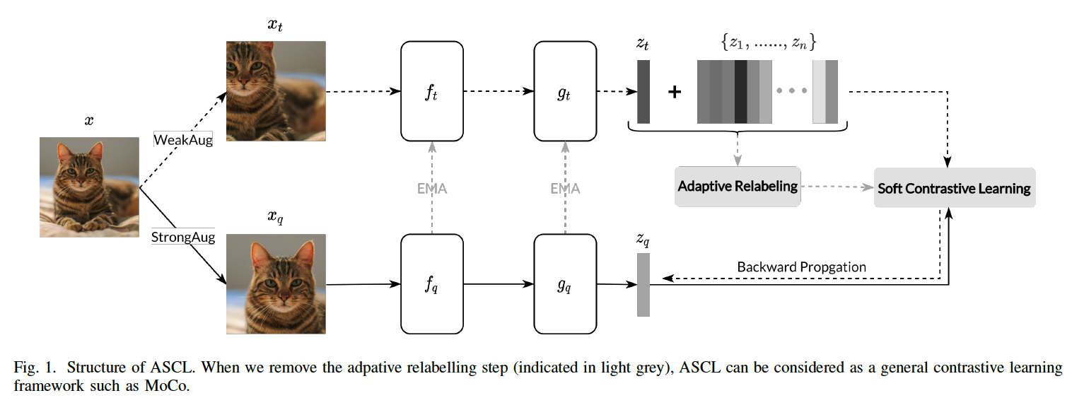
Instance discrimination task
- considering each image instance as a separate semantic class
Proposed method : use MoCo method
- given sample \(x\), generate 2 views
- query \(x_q\)
- target \(x_t\)
- Goal :
- minimize the distance of \(z_q\) and \(z_t\)
- maximize the distance of \(z_q\) and representations of other samples cached in a memory bank \(\left\{z_1, \ldots, z_n\right\}\).
- Model :
- encoders \(f_q, f_t\) and projectors \(g_q, g_t\)
- \(z_{-}=g\left(f\left(x_{-}\right)\right)\).
InfoNCE loss :
\(L=-\log \frac{\exp \left(z_q^T z_t / \tau\right)}{\exp \left(z_q^T z_t / \tau\right)+\sum_{i=1}^n \exp \left(z_q^T z_i / \tau\right)}\).
(1) Soft contrastive learning
Combine \(z_t\) and memory bank \(\left\{z_1, \ldots, z_n\right\}\)
\(\rightarrow\) \(\left\{z_1^{\prime}, z_2^{\prime}, \ldots, z_{n+1}^{\prime}\right\} \triangleq\left\{z_t, z_1, \ldots, z_n\right\}^1\), we can easily rewrite
Rewrite InfoNCE as …
- (Before) \(L=-\log \frac{\exp \left(z_q^T z_t / \tau\right)}{\exp \left(z_q^T z_t / \tau\right)+\sum_{i=1}^n \exp \left(z_q^T z_i / \tau\right)}\).
- (After) \(L=-\sum_{j=1}^{n+1} y_j \log p_j\)
- where \(p_j=\frac{\exp \left(z_q^T z_j^{\prime} / \tau\right)}{\sum_{i=1}^{n+1} \exp \left(z_q^T z_i^{\prime} / \tau\right)}\)
- \(\boldsymbol{p}=\left[p_1, \ldots, p_{n+1}\right]\) is the prediction probability vector
- where \(y_j= \begin{cases}1, & j=1 \\
0, & \text { otherwise }\end{cases}\).
- \(\boldsymbol{y}=\left[y_1, \ldots, y_{n+1}\right]\) is the one-hot pseudo label
- where \(p_j=\frac{\exp \left(z_q^T z_j^{\prime} / \tau\right)}{\sum_{i=1}^{n+1} \exp \left(z_q^T z_i^{\prime} / \tau\right)}\)
By modifying pseudo label, convert “original” CL \(\rightarrow\) “soft” CL
(2) Adaptive Relabeling
the pseudo label in infoNCE loss
\(\rightarrow\) ignores the inter-sample relations which will result in false negatives (FN)
Modify the pseudo label
- based on the neighboring relations in the feature space
- step 1) calculate the cosine similarity \(\boldsymbol{d}\)
- between self positive view \(z_1^{\prime}\) & representations in memory bank \(\left\{z_2^{\prime}, z_3^{\prime}, \ldots, z_{n+1}^{\prime}\right\}\)
- \(d_j=\frac{z_1^{\prime T} z_j^{\prime}}{ \mid \mid z_1^{\prime} \mid \mid _2 \mid \mid z_j^{\prime} \mid \mid _2}, j=2, \ldots, n+1\).
- step 2)
- a) Hard Relabeling
- b) Adaptive Hard Relabeling
- c) Adaptive Soft Relabeling
a) Hard Relabeling
-
according to \(d_j, i=2, \ldots, n+1\),
define the top- \(K\) nearest neighbors set \(\mathcal{N}_K\) in the memory bank of \(z_1^{\prime}\)
- treat them as extra positives for \(z_q\).
- NEW pseudo label \(\boldsymbol{y}_{\text {hard }}\) :
- \(y_j=\left\{\begin{array}{l} 1, j=1 \text { or } z_j \in \mathcal{N}_K \\ 0, \text { otherwise } \end{array}\right.\).
- summary ) positive for \(z_q\)
- (1) \(z_1^{\prime}\)
- (2) top- \(K\) nearest neighbors of \(z_1^{\prime}\).
b) Adaptive Hard Relabeling
Risky to recklessly assume that the top- \(K\) nearest neighbors are positive
\(\rightarrow\) propose an adaptive mechanism that automatically modifies the confidence of the pseudo label.
with cosine similarity \(d\) ,
build the relative distribution \(\boldsymbol{q}\) between ..
- (1) self positive view \(z_1^{\prime}\)
- (2) other representations in memory bank \(\left\{z_2^{\prime}, z_3^{\prime}, \ldots, z_{n+1}^{\prime}\right\}\)
\(q_j=\frac{\exp \left(d_j / \tau^{\prime}\right)}{\sum_{l=2}^{n+1} \exp \left(d_l / \tau^{\prime}\right)}, j=2, \ldots, n+1\).
Uncertainty of relative distribution
\(c=1-\frac{H(\boldsymbol{q})}{\log (n)}\).
- define a confidence measure as the normalized entropy of the distribution \(q\)
- \(H(\boldsymbol{q})\) : Shannon entropy
- \(\log (n)\) : to normalize \(c\) into [0,1]
Adaptive hard label \(\boldsymbol{y}_{\text {ahcl }}\)
- by augmenting \(\boldsymbol{y}_{\text {hard }}\) with \(c\)
- \(y_j=\left\{\begin{array}{l} 1, j=1 \\ c, j \neq 1 \text { and } z_j \in \mathcal{N}_K \\ 0, j \neq 1 \text { and } z_j \notin \mathcal{N}_K \end{array}\right.\).
c) Adaptive Soft Relabeling
instead of using top- \(K\) neighbors …
\(\rightarrow\) propose using the distribution \(\boldsymbol{q}\) itself as soft labels.
Adaptive soft label \(\boldsymbol{y}_{\text {ascl }}\) :
- \(y_j=\left\{\begin{array}{l}
1, j=1 \\
\min \left(1, c \cdot K \cdot q_j\right), j \neq 1
\end{array}\right.\).
- \(c=1-\frac{H(\boldsymbol{q})}{\log (n)}\).
- \(K\) : number of neighbors in \(\mathcal{N}_K\).
d) Common
\(\boldsymbol{y}_{a s c l}, \boldsymbol{y}_{a h c l}\) and \(\boldsymbol{y}_{\text {hard }}\) are then normalized : \(y_j=\frac{y_j}{\sum_{-} y_{-}}\).
(3) Distribution Sharpening
temperature \(\tau\) in infoNCE loss
- controls the density of the learned representations
- smaller temperature \(\tau^{\prime}\) :
- filter out possible noisy relations
- (default) \(\tau=0.1, \tau^{\prime}=0.05\)