CReST: A Class-Rebalancing Self-Training Framework for Imbalanced Semi-Supervised Learning

Abstract
Introduction
Related Work
1. Semi-SL
2. Class-imbalanced SL
3. Class-imbalanced Semi-SL
Class-imbalanced Semi-SL
1. Problem setup and baselines
2. A closer look at the model bias
3. Class-rebalancing self-training
4. Progressive Distribution Alignment
Experiments
1. CIFAR-LT
2. ImageNet127
3. Ablation Study

0. Abstract

[ Semi-SL on Imbalanced Data ]

Existing Semi-SL methods :

perform poorly on minority classes
still generate high precision pseudo-labels on minority classes.

Class- Rebalancing Self-Training (CReST),

Simple yet effective framework to improve existing Semi-SL methods on class imbalanced data.
Iteratively retrains a baseline Semi-SL model with a labeled set expanded by adding pseudo-labeled samples from an unlabeled set
- pseudo-labeled samples from minority classes are selected more frequently according to an estimated class distribution.
CResT+ : a progressive distribution alignment to adaptively adjust the rebalancing strength

1. Introduction

Semi-SL’s common assumption

= the class distribution of labeled and/or unlabeled data are balanced

\(\rightarrow\) Not in reality!

Supervised Leanring (on imbalanced data)

biased towards majority classes
various solutions have been proposed to help alleviate bias
- ex) re-sampling, re-weighting, two-stage training
\(\rightarrow\) rely on labels to rer-balance the biased model

Semi-SL (on imbalanced data)

has been under-studied
data imbalance poses further challenges in Semi-SL
- missing label information precludes rebalancing the unlabeled set.
Pseudo-labeling
- label for unlabeled data generated by a model trained on labeled data
- problematic if they are generated by an initial model trained on imbalanced data
Majority of existing Semi-SL algorithms have not been evaluated on imbalanced data distributions.

This paper : Semi-SL under class-imbalanced data

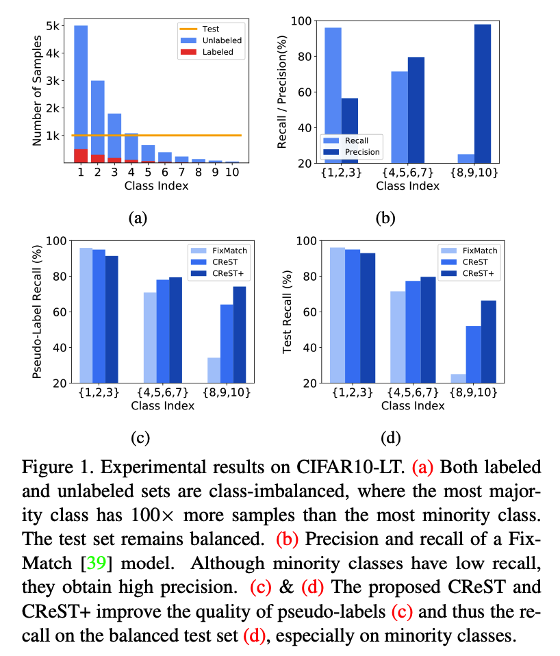
Undesired performance of existing Semi-SL algorithms on imbalanced data

\(\rightarrow\) Due to low recall on minority classes

( but note that …. precision on minority classes is surprisingly high !! )

suggest that the model is conservative in classifying samples into minority classes, but once it makes such a prediction we can be confident it is correct.

Class-rebalancing self-training scheme (CReST)

re-trains a baseline Semi-SL model after adaptively sampling pseudo-labeled data from the unlabeled set
Generation = fully-trained baseline model

After each generation, pseudo-labeled samples from the unlabeled set are added into the labeled set to retrain an Semi-SL model.
CReST
- update labeled set with ALL pseudo-labeled samples (X)
- use a stochastic update strategy (O)
  - samples are selected with higher probability if they are predicted as minority classes ( as those are more likely to be correct predictions )
Updating probability in CReST
- is a function of the data distribution estimated from the labeled set.
- extend CReST to CReST+ by incorporating distribution alignment with a temperature scaling factor
Figure 1-(c) & (d)

(1) Semi-SL

(2) Class-imbalanced supervised learning

a) Re-sampling & Re-weighting

re-balance the contribution of each class

b) Transfer knowledge from majority classes to minority classes.

c) Decouple the learning of representation & classifier

\(\rightarrow\) Assume all labels are available during training ( not on Semi-SL setting )

(3) Class-imbalanced semi-supervised learning

( Semi-SL : Underexplored under class-imbalanced data. )

Yang and Xu

leveraging unlabeled data by Semi-SL & SSL can benefit class-imbalanced learning.

Hyun et al.

proposed a suppressed consistency loss to suppress the loss on minority classes.

Kim et al.

proposed Distribution Aligning Refinery (DARP) to refine raw pseudo-labels via a convex optimization.

This paper : boost the quality of the model’s raw pseudo-labels directly via

(1) Class-rebalancing sampling strategy
(2) Progressive distribution alignment strategy

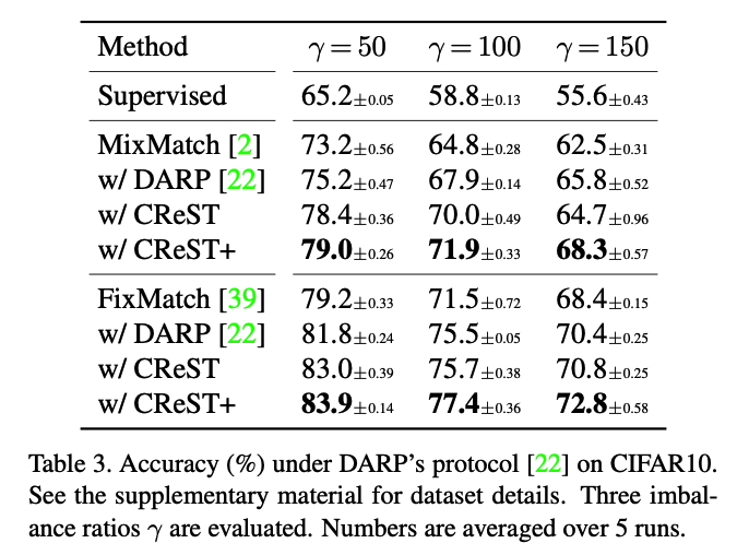
CReST vs. DARP

DARP : setting where labeled and unlabeled data do not share the same class
CReST : focus on the scenario when labeled and unlabeled data have roughly the same distribution.

3. Class-Imbalanced Semi-SL

(1) Problem setup and baselines

Class-imbalanced Semi-SL

\(L\)-class classification task
Dataset : \(\mathcal{X}=\left\{\left(x_n, y_n\right): n \in(1, \ldots, N)\right\}\)
- \(x_n \in \mathbb{R}^d\).
- \(y_n \in\{1, \ldots, L\}\).
\(N_l\) : Number of training examples in \(\mathcal{X}\) of class \(l\) ,
- \(\sum_{l=1}^L N_l=N\).
- \(N_1 \geq N_2 \geq \cdots \geq N_L\).
The marginal class distribution of \(\mathcal{X}\) is skewed ( \(N_1 \gg N_L\). )
Imbalance ratio : \(\gamma=\frac{N_1}{N_L}\).
Unlabeled set \(\mathcal{U}=\left\{u_m \in \mathbb{R}^d: m \in(1, \ldots, M)\right\}\)
- same class distribution as \(\mathcal{X}\)
Label fraction \(\beta=\frac{N}{N+M}\) : percentage of labeled data.

Goal : Given class-imbalanced sets \(\mathcal{X}\) and \(\mathcal{U}\), learn a classifier \(f: \mathbb{R}^d \rightarrow\{1, \ldots, L\}\) that generalizes well under a class-balanced test criterion.

SOTA Semi-SL methods

utilize unlabeled data by assigning a pseudo-label with the classifier’s prediction \(\hat{y}_m=f\left(u_m\right)\).
then, useboth labeled and unlabeled samples to train classifier

When the classifier is biased at the beginning due to a skewed class distribution…

\(\rightarrow\) online pseudo-labels of unlabeled data can be even more biased!

(2) A closer look at the model bias

Long-tailed versions of CIFAR

with various class-imbalanced ratios
to evaluate class-imbalanced fully-supervised learning algorithms.

This paper : follow the above protocol!

some as LABELED
some as UNLABELED

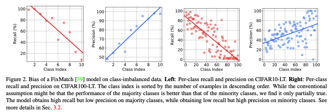
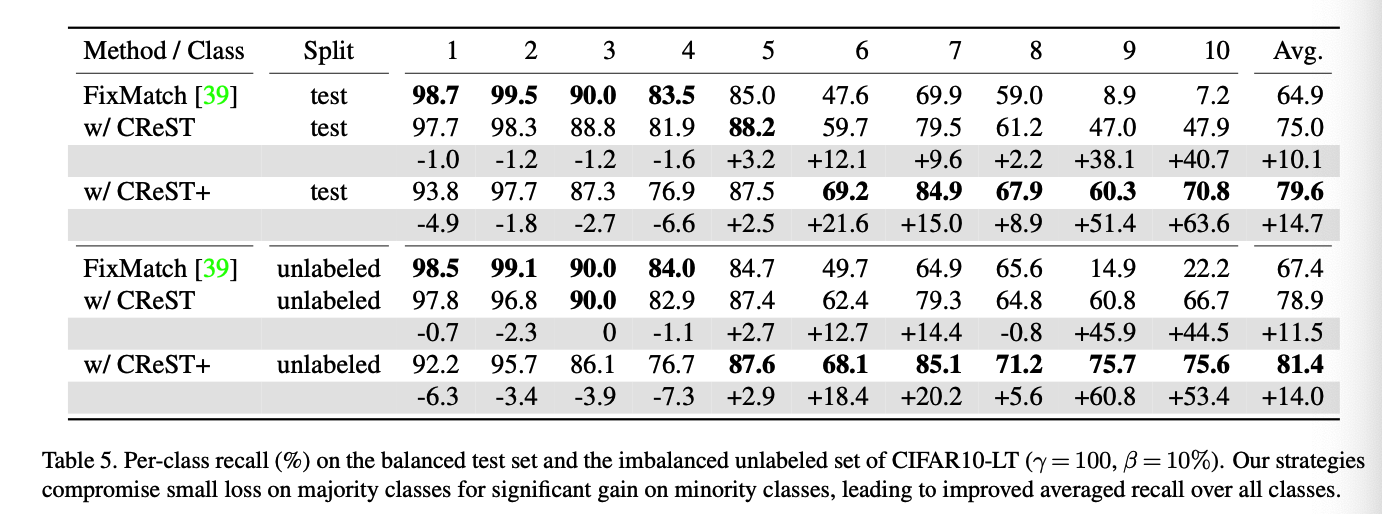
Despite the low recall, the minority classes maintain surprisingly high precision!!!

(3) Class-rebalancing self-training

Self-training

Iterative method widely used in Semi-SL.
- It trains the model for multiple generations, where each generation involves two steps.
Procedure
- step 1) Trained on the labeled set to obtain a teacher model
- step 2) Teacher model’s predictions are used to generate pseudo-labels \(\hat{y}_m\) for unlabeled data \(u_m\).
- step 3) Add to labeled set for the next generation.
  - \(\hat{\mathcal{U}}=\left\{\left(u_m, \hat{y}_m\right)\right\}_{m=1}^M\) .
  - \(\mathcal{X}^{\prime}=\mathcal{X} \cup \hat{\mathcal{U}}\),

To accommodate the class-imbalance….

Propose two modifications to the self-training strategy!

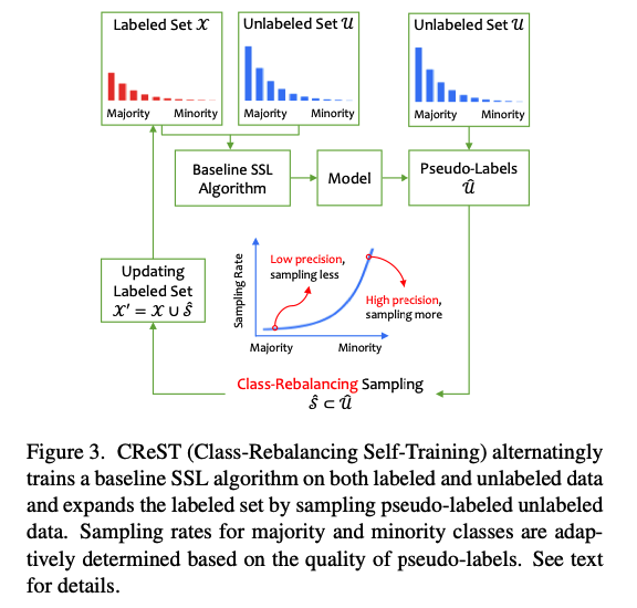
(1) Instead of solely training on the labeled data, use Semi-SL algorithms to exploit both labeled and unlabeled data to get a better teacher model in the first step.

(2) Rather than including every sample in \(\hat{\mathcal{U}}\) in the labeled set, we instead expand the labeled set with a selected subset \(\hat{\mathcal{S}} \subset \hat{\mathcal{U}}\), i.e., \(\mathcal{X}^{\prime}=\mathcal{X} \cup \hat{\mathcal{S}}\).

We choose \(\hat{\mathcal{S}}\) following a class-rebalancing rule:
- the less frequent a class \(l\) is, the more unlabeled samples that are predicted as class \(l\) are included into the pseudo-labeled set \(\hat{\mathcal{S}}\).

Class Distribution

estimate from labeled set
unlabeled samples that are predicted as class \(l\) are included into \(\hat{\mathcal{S}}\) at the rate of
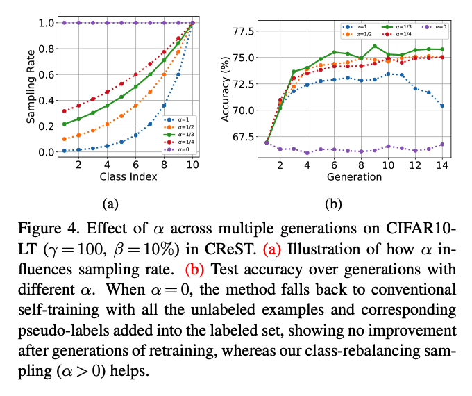
- \(\mu_l=\left(\frac{N_{L+1-l}}{N_1}\right)^\alpha\).
  - \(\alpha \geq 0\) : tunes the sampling rate
Ex) 10-class imbalanced dataset with imbalance ratio of \(\gamma=\frac{N_1}{N_{10}}=100\),
- samples predicted as the most minority class
  - keep all ! … \(\mu_{10}=\left(\frac{N_{10+1-10}}{N_1}\right)^\alpha=1\).
- samples predicted as the most majority class
  - Only \(\mu_1=\left(\frac{N_{10+1-1}}{N_1}\right)^\alpha=0.01^\alpha\) of samples are selected.
When \(\alpha=0, \mu_l=1\) for all \(l\), then all unlabeled samples are kept and the algorithm falls back to the conventional self-training.

When selecting pseudo-labeled samples in each class, we take the most confident ones.

Motivation of our CReST strategy

Precision of minority classes is much higher than that of majority classes
- minority class pseudo-labels are less risky to include in the labeled set.
Adding samples to minority classes is more critical due to data scarcity.

(4) Progressive Distribution Alignment

Improve the quality of online pseudo-labels …

by additionally introducing progressive distribution alignment into CReST

=> CReST +

Distribution Alignment (DA)

introduced for class-balanced Semi-SL

( also fits with also for class-imbalanced ! )
aligns the model’s predictive distribution ( on unlabeled samples )

with the labeled training set’s class distribution \(p(y)\).

\(\tilde{p}(y)\) : MA of the model’s predictions on unlabeled examples.

Procedure of DA

Step 1) Scales the model’s prediction \(q=p\left(y \mid u_m ; f\right)\) for an unlabeled example \(u_m\) by the ratio \(\frac{p(y)}{\tilde{p}(y)}\)

( = aligning \(q\) with the target distribution \(p(y)\). )
Step 2) Re-normalizes the scaled result
- \(\tilde{q}=\operatorname{Normalize}\left(q \frac{p(y)}{\tilde{p}(y)}\right)\), where Normalize \((x)_i=x_i / \sum_j x_j\).
- use \(\tilde{q}\) instead of \(q\) for the label guess for \(u_m\)

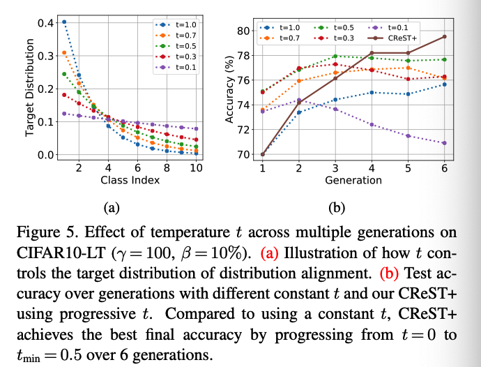
Progressive DA

use temperature scaling to enhance DA’s ability to handle class-imbalanced data
add a tuning knob \(t \in[0,1]\)
- controls the class-rebalancing strength of DA.
Use \(\operatorname{Normalize}\left(p(y)^t\right)\) instead of \(p(y)\) as target,
- When \(t=1\), same as original DA
- When \(t<1\), the taget distn becomes smoother and balances the model’s predictive distribution more aggressively.
- When \(t=0\), the target distribution becomes uniforrm

Pogressively increase the strength of class-rebalancing by decreasing \(t\) over generations.

\(t_g=\left(1-\frac{g}{G}\right) \cdot 1.0+\frac{g}{G} \cdot t_{\min }\).
- \(G+1\) : total number of generations
- \(t_{\min }\) : temperature used for the last generation
Enjoys both
- high precision of pseudo-labels in early generations
- stronger class-rebalancing in late generations.

4. Experiments

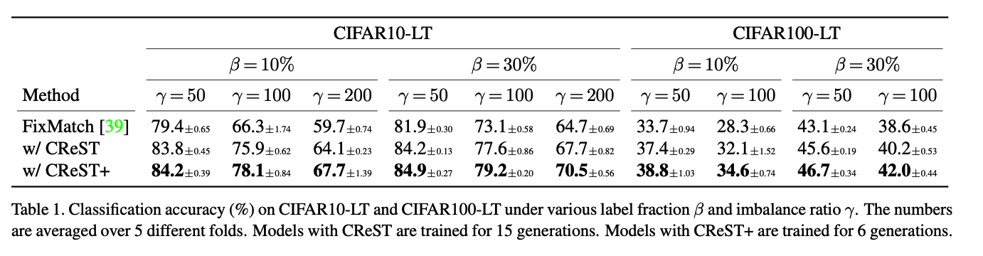
(1) CIFAR-LT

Datasets

CIFAR10-LT
CIFAR100-LT

Training images

randomly discarded per class
pre-defined imbalance ratio \(\gamma\).
\(N_l=\gamma^{-\frac{l-1}{L-1}} \cdot N_1\) .
- (CIFAR10-LT) \(N_1=5000, L=10\)
- (CIFAR100-LT) \(N_1=500, L=100\)

Experimental Settings

(1) Unlabeled ratio : \(\beta\)
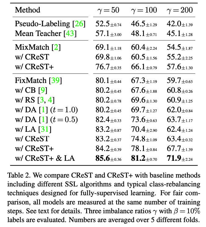
- Randomly select \(\beta=10 \%\) and \(30 \%\) of samples from training data as labeled set
(2) Imbalance ratio : \(\gamma\)
- (CIFAR10-LT) \(\gamma\) = 50, 100, 200
- (CIFAR100-LT) \(\gamma\) = 50, 100

Testing images

remains untouched
balanced ( thus evaluated criterion is on class-balanced dataset )

a) Main Results

b) Comparison with baselines

c) Comparison with DARP

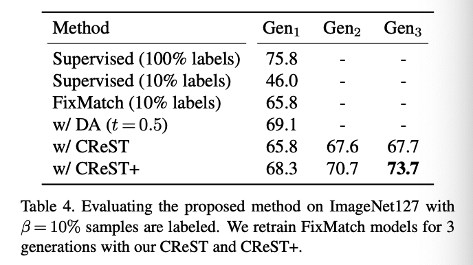
(2) ImageNet127

Dataset

Large-scale datasets.
1000 classes of ImageNet \(\rightarrow\) Grouped into 127 classes
- based on their top-down hierarchy in WordNet.
Imbalanced dataset
- with imbalance ratio \(\gamma=286\).
- Majority Class : “mammal”
  - consists of 218 original classes
  - 277,601 training images.
- Minority Class : “butterfly”
  - single original class
  - 969 training examples.