
Self-Damaging Contrastive Learning
Contents
- Abstract
- Introduction
- Background & Research Gaps
- Rationale and Contributions
- Related Works
- Data Imbalance and SSL
- Pruning as Compression and Beyond
- Contrasting Different Models
- Methods
- Preliminaries
- Self-Damaging Contrastive Learning
- More Discussion on SDCLR
- Experiments
- Datasets & Training Settings
0. Abstract
Unlabeled data in reality
- imbalanced & long-tail distribution,
\(\rightarrow\) Unclear how robustly the latest CL methods could perform
Hypothesize that long-tail samples are also tougher for the model to learn well due to **insufficient examples
Self-Damaging Contrastive Learning (SDCLR),
-
to automatically balance the representation learning without knowing the classes.
-
create a dynamic self-competitor model to contrast with the target model,
( = pruned version of the target model )
-
contrasting the two models
\(\rightarrow\) lead to adaptive online mining of the “most easily forgotten samples” for the current target model,
& implicitly emphasize them more in the contrastive loss.
1. Introduction
(1) Background & Research Gaps
Contrastive learning
- learn powerful visual representations from unlabeled data.
- SOTA CL : consistently benefit from using bigger models and training on more task-agnostic unlabeled data
- ex) internet-scale sources of unlabeled data.
However, GAP between
- (1) “controlled” benchmark data
- (2) “uncontrolled” real-world data
Questions) Can CL can still generalize well in those LONG-TAIL scenarios?
- not the first to ask this question
- Earlier works (Yang \& Xu, 2020; Kang et al., 2021)
- when the data is imbalanced by class, CL can learn more balanced feature space than SL
Find that SOTA CL methods remain certain vulnerability to the long-tailed data
-
reflected on the linear separability of pretrained features
-
instance-rich classes = much more separable features
( than instance-scarce classes )
-
-
BUT … CL does not use class (label) information ! Then HOW ??
(2) Rationale and Contributions
Overall goal : Extend the (a) loss re-balancing and (b) cost-sensitive learning ideas into an unsupervised setting.
Previous findings:
- Network pruning = removes the smallest magnitude weights in a trained DNN
- affect all learned classes or samples unequally
- forget LONG-tailed and most difficult images more!
\(\rightarrow\) Inspired this .. propose Self-Damaging Contrastive Learning (SDCLR)
- to automatically balance the representation learning without knowing the classes
Details
-
strong contrastive views by input data augmentation
-
new level of contrasting via“model augmentation”
- by perturbing the target model’s structure and/or current weights.
-
**Dynamic self-competitor model **
( = by pruning the target model online )
- contrast the pruned model’s features with the target model’s.
-
Rare Instances
= largest prediction differences between pruned & non-pruned models.
Since the self-competitor is always obtained from the updated target model, the two models will co-evolve
\(\rightarrow\) allows the target model to spot diverse memorization failures at different training stages and to progressively learn more balanced representations.
2. Related Works
(1) Data Imbalance and SSL
Classical LT recognition
- mainly amplify the impact of TAIL class samples
- ex) re-sampling or re-weighting
\(\rightarrow\) Rely on label information & not directly applicable to unsupervised representation learning
Kang et al., 2019; Zhang et al., 2019
-
learning of (1) feature extractor and (2) classifier head can be decoupled.
( = pre-training a feature extractor )
Yang \& Xu, 2020
-
Benefits of a balanced feature space from SSL pre-training for generalization.
-
first study to utilize SSL for overcoming the intrinsic label bias.
- SSL pre-training » end-to-end baselines
- given more unlabeled data, the labels can be more effectively leveraged in a semi-supervised manner for accurate and debiased classification. reduce label bias in a semi-supervised manner.
Kang et al., 2021
- ( when the data is imbalanced by class ) CL can learn more balanced feature space than SL
(2) Pruning as Compression and Beyond
Frankle \& Carbin, 2018
- showed that there exist highly sparse “critical subnetworks” from the full DNNs,
- This critical subnetwork could be identified by iterative unstructured pruning (Frankle et al., 2019).
Hooker et al., 2020
- For a trained image classifier, pruning it has a “NON-uniform” impact
- disproportionately impacted by the introduction of sparsity.
- Wang et al., 2021
- leveraged this idea
- construct an ensemble of self-competitors from one dense model
(3) Contrasting Different Models
High-level idea of SDCLR
= contrasting two similar competitor models & weighing more on their most DISAGREED samples
Co-teaching (Han et al., 2018; Yu et al., 2019)
-
performs sample selection in noisy label learning by using two DNNs
- each trained on a different subset of examples that have a small training loss for the other network
-
Limitation : examples that are selected tend to be easier
\(\rightarrow\) slow down learning & and hinder generalization to more difficult data
SDCLR : designed to focus on the difficult-to-learn samples in the long tail.
3. Methods
(1) Preliminaries
a) Contrastive Learning
- pass
b) Pruning Identified Exemplars
Hooker et al., 2020
- systematically investigates the model output changes introduced by pruning
- finds that certain examples are particularly sensitive to sparsity
- Pruning Identified Exemplars (PIEs) = most affected instance
- difficult-to-memorize samples in training.
- demonstrate that PIEs often show up at the long-tail of a distribution.
This paper extend PIE hypothesis from “SL” to “SSL”
-
Instead of pruning a trained model and expose its PIEs once,
integrate pruning into the training process as an online step.
-
With PIEs dynamically generated by pruning a target model under training, we expect them to expose different long-tail examples during training
( \(\because\) the model continues to be trained )
(2) Self-Damaging Contrastive Learning
CL is NOT immune to imbalance
- Even CL does not rely on class labels, it still learns the transformation invariances in a data-driven manner, and will be affected by dataset bias (Purushwalkam \& Gupta, 2020).
Kang et al., 2021
- using the CL can obtain a balanced representation space that has similar separability for all the classes,
- experiments on ImageNet-LT & iNaturalist
However, this paper point out that it was pre-mature to conclude “contrastive learning is immune to imbalance”.
-
shown in experriments in Section 4.3
( have constructed a few heavily imbalanced data settings, where CL will become unable to produce balanced features )
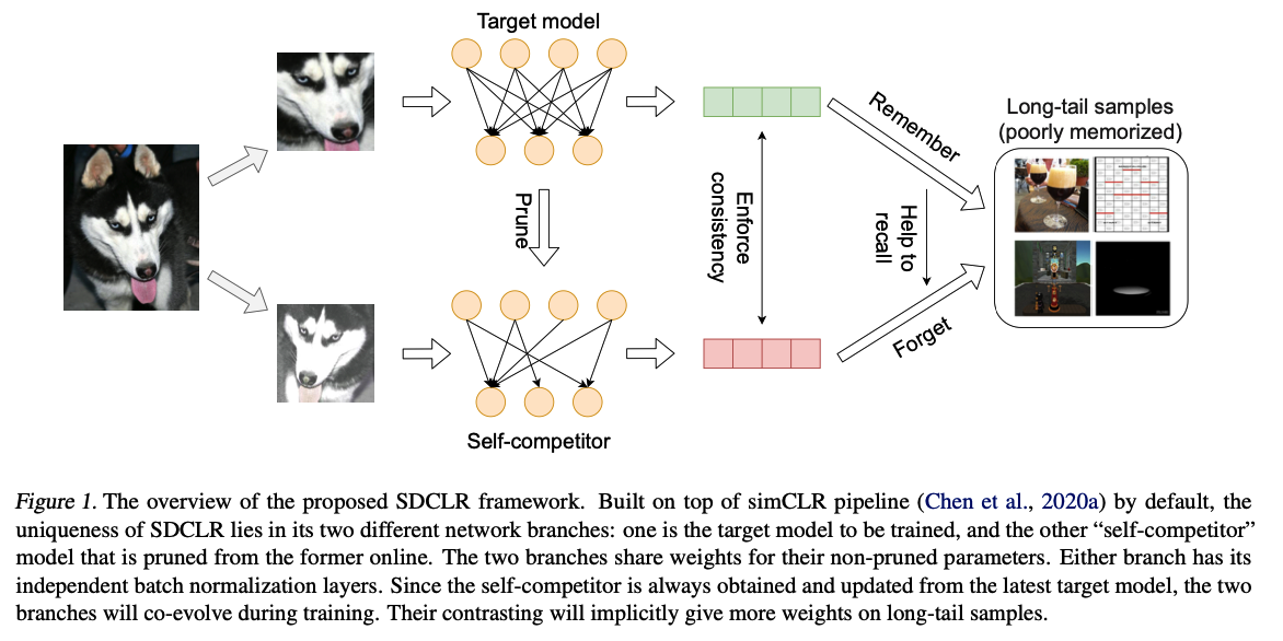
SDCLR Framework
Overview
- Built on top of the SimCLR pipeline
- Main difference between SimCLR :
- SimCLR : same target network backbone (via weight sharing);
- SDCLR : creates a “self-competitor”
- by pruning the target model online
- lets the two different branches take the two augmented images
Details
-
at each iteration ) have a…
- (1) Dense branch \(N_1\)
- (2) Sparse branch \(N_2^p\) ( by pruning \(N_1\) )
using the simplest magnitude-based pruning
-
Pruning mask of \(N_2^p\) could be updated per iteration after the model weights are updated.
-
Since the backbone is a large DNN and its weights will not change much for a single iteration or two,
\(\rightarrow\) Set the pruning mask to be lazy-updated at the beginning of every epoch, to save computational overheads;
- all iterations in the same epoch then adopt the same mask
-
self-competitor is always obtained and updated from the latest target model
\(\rightarrow\) the two branches will co-evolve during training.
Notation
- input image \(I\)
- two different versions \(\left[\hat{I}_1, \hat{I}_2\right]\).
- encoder : \(\left[N_1, N_2^p\right]\)
- share the same weights in the non-pruned part
- \(N_1\) will independently update the remaining part
- output features : \(\left[f_1\right.\), \(f_2^p\) ]
- fed into the nonlinear projection heads to enforce similarity be under the NT-Xent loss
If the sample is well-memorized by \(N_1\), pruning \(N_1\) will not “forget” it
For RARE ( atypical ) instances …
SDCLR will amplify the prediction differences
- between the (1) pruned and (2) non-pruned models
\(\rightarrow\) Hence those samples’ weights be will implicitly increased in the overall loss.
( + it helps to let either branch have its independent BN layers )
(3) More Discussion on SDCLR
SDCLR can work with more CL frameworks
- SDCLR = plug-and-play
- any architectuer adopting the the two-branch design
Pruning is NOT for model efficiency in SDCLR
- NOT using pruning for any model efficiency purpose
- better described as “selective brain damage”.
- for effectively spotting samples not yet well memorized and learned by the current model.
- “side bonus” : sparsity itself can be an effective regularizer
SDCLR benefits beyond standard class imbalance.
- can be extended seamlessly beyond the standard single-class label imbalance case.
- ex) multi-label attribute imbalance
- more inherent forms of “imbalance”
- ex) class-level difficulty variations or instance-level feature distributions
4. Experiments
(1) Datasets & Training Settings
Three popular imbalanced datasets
- (1) long-tail CIFAR-10
- (2) long-tail CIFAR-100
- (3) ImageNet-LT
+ Consider a more realistic and more challenging benchmark, long-tail ImageNet-100
- with a different exponential sampling rule.
- contains less classes
- which decreases the number of classes that looks similar and thus can be more vulnerable to imbalance.
a) Long-tail CIFAR10/CIFAR100
Original CIFAR
- consist of 60000 32 \(\times\) 32 images in 10/100 classes.
Long tail CIFAR
-
first introduced in (Cui et al., 2019)
-
by sampling long tail subsets from the original datasets.
-
Imbalance factor = class size of the largest class / smallest class
( default : set it to 100 )
-
to alleviate randomness … conduct on 5 different LT sub-samplings
b) ImageNet-LT
The sample number of each class :
\(\rightarrow\) determined by a Pareto distribution with the power value \(\alpha=6\).
Contains \(115.8 \mathrm{~K}\) images,
- number per class : ranging from 1280 to 5
c) ImageNet-LT-exp
Given by an exponential function
- Imbalanced factor = 256
- minor class scale is the same as ImageNet-LT.
Contains \(229.7 \mathrm{~K}\) images
d) Long tail ImageNet-100
Dataset with a small scale and large resolution.
ImageNet-100-LT :
- from ImageNet-100
- sample number of each class : determined by a down-sampled (from 1000 classes to 100 classes) Pareto distribution used for ImageNet-LT.
Contains \(12.21 \mathrm{~K}\) images
- number per class : ranging from 1280 to 5