
( 참고 : 패스트 캠퍼스 , 한번에 끝내는 컴퓨터비전 초격차 패키지 )
LeNet & AlexNet & VGG
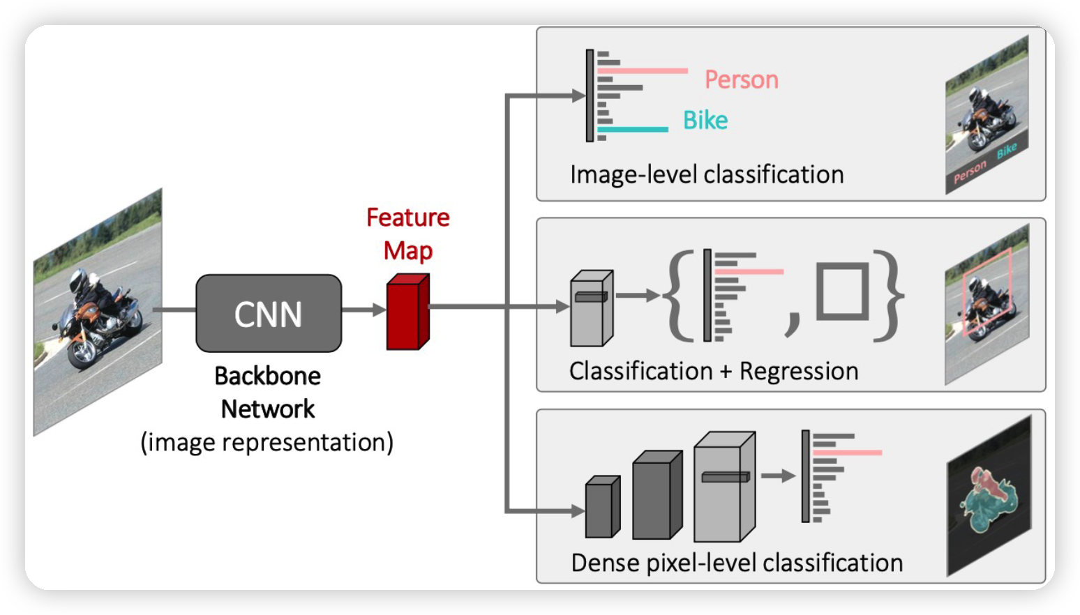
기본적인 CNN구조는 여러 task에 대한 backbone 역할을 한다.
- 이미지의 공통적인 특징을 추출하는 역할!
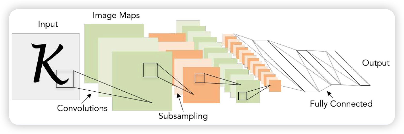
1. LeNet
- by Yann LeCun (1998)
- 가장 기본적인 CNN 아키텍처
- convolution : 5x5 필터 ( stride=1 )
- max pooling : 2x2 ( stride=2 )
2. AlexNet
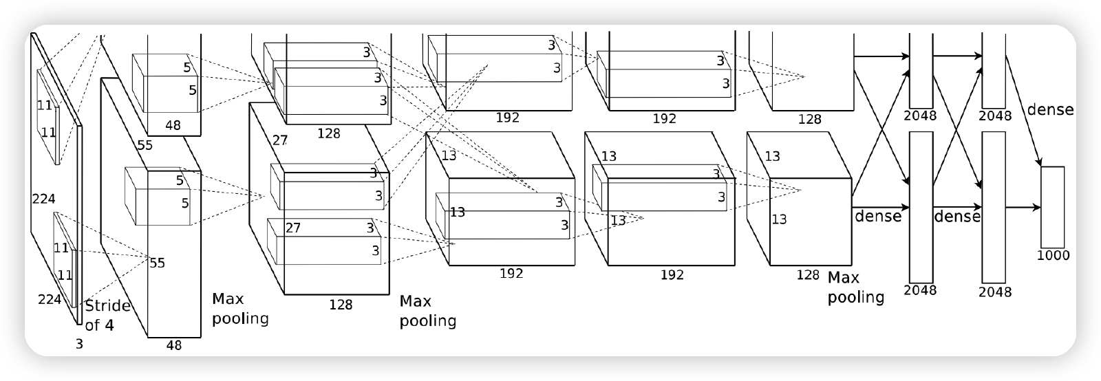
- LeNet과의 차이점 :
- 7개의 hidden layer, 650k 뉴런, 6000만개의 파라미터
- ImageNet으로 학습
- ReLU & Dropout 사용
3. VGG
- 깊은 layer ( 16 & 19 )
- 간단한 아키텍처
- 3x3 convolution filter만 사용함 ( stride=1 )
- 2x2 max pooling
4. 코드 실습
(1) Import Packages
import torch, torchvision
import torchvision.models as models

import matplotlib.pyplot as plt
from PIL import Image
(2) Import Pre-trained Models
그 구조를 확인해보자면…
models.alexnet(pretrained=False)
# models.vgg11()
# models.vgg11_bn()
# models.vgg19()
AlexNet(
  (features): Sequential(
    (0): Conv2d(3, 64, kernel_size=(11, 11), stride=(4, 4), padding=(2, 2))
    (1): ReLU(inplace=True)
    (2): MaxPool2d(kernel_size=3, stride=2, padding=0, dilation=1, ceil_mode=False)
    (3): Conv2d(64, 192, kernel_size=(5, 5), stride=(1, 1), padding=(2, 2))
    (4): ReLU(inplace=True)
    (5): MaxPool2d(kernel_size=3, stride=2, padding=0, dilation=1, ceil_mode=False)
    (6): Conv2d(192, 384, kernel_size=(3, 3), stride=(1, 1), padding=(1, 1))
    (7): ReLU(inplace=True)
    (8): Conv2d(384, 256, kernel_size=(3, 3), stride=(1, 1), padding=(1, 1))
    (9): ReLU(inplace=True)
    (10): Conv2d(256, 256, kernel_size=(3, 3), stride=(1, 1), padding=(1, 1))
    (11): ReLU(inplace=True)
    (12): MaxPool2d(kernel_size=3, stride=2, padding=0, dilation=1, ceil_mode=False)
  )
  (avgpool): AdaptiveAvgPool2d(output_size=(6, 6))
  (classifier): Sequential(
    (0): Dropout(p=0.5, inplace=False)
    (1): Linear(in_features=9216, out_features=4096, bias=True)
    (2): ReLU(inplace=True)
    (3): Dropout(p=0.5, inplace=False)
    (4): Linear(in_features=4096, out_features=4096, bias=True)
    (5): ReLU(inplace=True)
    (6): Linear(in_features=4096, out_features=1000, bias=True)
  )
)
pre-trained 모델 불러오기 (with weight)
alexnet = models.alexnet(pretrained=True)

alexnet.eval() # FREEZE
alexnet.train() # Trainable
(3) Example
a) Import Dataset
image = './data/house.jpg'
image = Image.open(image).convert('RGB')
b) Pre-processing
-
torchvision.transforms사용 -
(1) 텐서 변환
-
(2) 정규화
-
R/G/B각각 스케일이 다르다. 따라서, (ImageNet데이터의 R/G/B에 맞는)
- 평균 : 0.485, 0.456, 0.406
- 표준편차 : 0.229, 0.224, 0.225
로 정규화해준다.
-
-
(3) Batchify
-
input으로 받는 데이터는 4차원이다.
( 첫 번째 차원은 “배치 차원”이다. 따라서, 맨 앞에 차원을 하나 추가해준다. )
-
to_tensor = torchvision.transforms.ToTensor()
normalizer = torchvision.transforms.Normalize(mean=[0.485, 0.456, 0.406],
                                 std=[0.229, 0.224, 0.225])

image = normalizer(to_tensor(image)) # 크기 : (3,1135,1920)
image = image.unsqueeze(0) # 크기 : (1, 3,1135,1920)
혹은, 아래와 같이 한번에 변환 가능
to_tensor = torchvision.transforms.Compose([
                torchvision.transforms.ToTensor(),
                torchvision.transforms.Normalize(mean=[0.485, 0.456, 0.406],
                                                 std=[0.229, 0.224, 0.225])])
(4) Output 확인
print("input shape: ", image.shape) # [1, 3, 1135, 1920]

#------------------------------------------------------------------------#
logit = alexnet(image)
print("output shape",logit.shape, logit) # [1, 1000]
print(torch.argmax(logit)) # 660
(5) 데이터셋 불러오기
Ex) CIFAR10 데이터셋
cifar10 = torchvision.datasets.CIFAR10(root='./', download=True)

print(len(cifar10)) # 50000
일반적인 Dataset과 마찬가지로, DataLoader로써 불러올 수 있다.
bs = 32

dataloader = torch.utils.data.DataLoader(cifar10,
                                         batch_size=bs,
                                         shuffle=True,
                                         num_workers=2)