
Universal Domain Adaptation ( 2019, 154 )
Contents
- Abstract
- Introduction
- Related Work
- Closed set DA
- Partial DA
- Open set DA (OSDA)
- Universal Domain Adaptation (UDA)
- Problem Setting
- Technical Challenges
- UAN (Universal Adaptation Network)
- Transferability Criterion
0. Abstract
UDA (Universal Domain Adaptation)
-
requires “no prior knowledge” on lael sets
- common label sets
- private label
\(\rightarrow\) allow category gap
-
requires a model to either
- (1) classify the target sample ( if associated with common label set )
- (2) mark it as “unknown” ( o.w )
\(\rightarrow\) propose UAN (Universal Adaptation Network)
1. Introduction
Existing DA algorithms : tackle the domain gap, by..
- 1) learning domain invariant feature representation
- 2) generating features/samples for target domains
- 3) transforming samples between domains, through generative models
2 Challenges
- 1) domain gap
- 2) category gap
UDA (Universal Domain Adaptation)
-
given a “labeled” source domain,
-
classify target data correctly, if it belongs to class in source label set,
or else mark it as “unknown”
2 Major challenges
- 1) cannot decide which part of source domain should be matched to which part of target domain
- 2) should be able to target some as “unknown”
UAN (Universal Adaptation Network)
-
quantify the transferability of each sample
-
criterion integrates both…
- 1) domain similarity
- 2) prediction uncertainty
2. Related Work
According to the “constraint on the label set” relationship between domain…
- 1) closed set DA
- 2) partial DA
- 3) open set DA
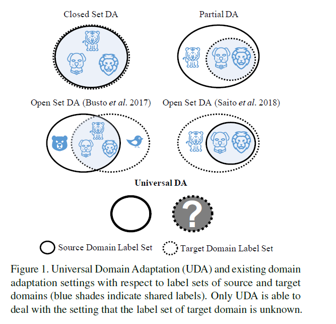
(1) Closed set DA
-
only deal with “domain gap”
-
fall into 2 categories
- 1) feature adaptation
- 2) generative model
a) feature adaptation
diminish the feature distribution discrepancy between 2 domains
examples )
-
minimize MMD of deep features across domains
( MMD = Maximum Mean Discrepancy )
-
residual transfer structure & entropy minimization on target data
-
distribution alignment by optimizing CMD
( CMD = Central Moment Discrepancy )
-
construct bipartite graph to force feature distribution alignment within clusters
-
DA by minimizing EMD
( Earth Mover’s Distance )
b) generative model
learn a domain classifier to discriminate features from source & target domains
\(\rightarrow\) force the feature extractor to confuse the domain classifier ( adversarial learning paradigm )
(2) Partial DA
examples)
- multiple domain discriminators with class-level & instance-level weighting mechanism
- auxiliary domain discriminator to quantify the **probability of source sample being similar to the target domain **
- only one adversarial network & jointly applying class-level weighting on the source classifier
(3) Open set DA (OSDA)
class private to both domains are unified as “unknown” class
3. Universal Domain Adaptation (UDA)
(1) Problem Setting
Notation
- source domain : \(\mathcal{D}_{s}=\left\{\left(\mathbf{x}_{i}^{s}, \mathbf{y}_{i}^{s}\right)\right\}\)
- distribution of source data : \(p\)
- \(p_{\mathcal{C}_{s}}\) : distribution of source data with labels in \(C_s\)
- \(p_{\mathcal{C}}\) : ~ in \(C\)
- \(C_s\) : label set of source domain
- distribution of source data : \(p\)
- target domain : \(\mathcal{D}_{t}=\left\{\left(\mathrm{x}_{i}^{t}\right)\right\}\)
- distribution of target data : \(q\)
- \(q_{\mathcal{C}_{t}}\) : distribution of target data with labels in \(C_t\)
- \(q_{\mathcal{C}}\) : ~ in \(C\)
- \(C_t\) : label set of target domain
- distribution of target data : \(q\)
- Common label set : \(\mathcal{C}=\mathcal{C}_{s} \cap \mathcal{C}_{t}\)
- Private label set :
- \(\overline{\mathcal{C}}_{s}=\mathcal{C}_{s} \backslash \mathcal{C}\).
- \(\overline{\mathcal{C}}_{t}=\mathcal{C}_{t} \backslash \mathcal{C}\).
Commonness between 2 domains
\(\xi=\frac{ \mid \mathcal{C}_{s} \cap \mathcal{C}_{t} \mid }{ \mid \mathcal{C}_{s} \cup \mathcal{C}_{t} \mid }\). ……… closed set DA : \(\xi=1\)
Task for UDA
= design a model that does not know \(\xi\), but works well across a wide spectrum of \(\xi\)
Goal : \(\min \mathbb{E}_{(\mathbf{x}, \mathbf{y}) \sim q_{\mathcal{C}}}[f(\mathbf{x}) \neq \mathbf{y}]\)
(2) Technical Challenges
a) “Category Gap” = difference of label sets
( “Domain Gap” still exists! That is, \(p \neq q\) & \(p_C \neq q_C\) )
b) detecting “unknown” classes
- low classification confidence
(3) UAN (Universal Adaptation Network)
Consists of 4 parts
- 1) feature extractor :\(F\)
- 2) adversarial domain discriminator : \(D\)
- 3) non-adversarial domain discriminator : \(D^{'}\)
- 4) label classifier : \(G\)
Process
- step 1) input \(\mathbf{x}\) is fed into \(F\) ….. \(\mathbf{z}=F(\mathbf{x})\)
- step 2)
- step 2-1) \(\mathbf{z}\) is fed into \(G\), to obtain “probability of class” over \(C_s\) ….. \(\mathbf{\hat{y}} = G(\mathbf{z})\)
- step 2-2) \(\mathbf{z}\) is fed into \(D^{'}\), to obtain “domain similarity” ….. \(\hat{d^{'}} = D(\mathbf{z^{'}})\)
- step 2-3) \(\mathbf{z}\) is fed into \(D\), to match feature distn of source & target ….. \(\hat{d} = D(\mathbf{z})\)
Error (Loss Function) : \(E_G, E_{D^{'}}, E_D\)
- \(E_{G} =\mathbb{E}_{(\mathbf{x}, \mathbf{y}) \sim p} L(\mathbf{y}, G(F(\mathbf{x})))\).
- \(E_{D^{\prime}}=-\mathbb{E}_{\mathbf{x} \sim p} \log D^{\prime}(F(\mathbf{x})) -\mathbb{E}_{\mathbf{x} \sim q} \log \left(1-D^{\prime}(F(\mathbf{x}))\right)\).
- \(E_{D}=-\mathbb{E}_{\mathbf{x} \sim p} w^{s}(\mathbf{x}) \log D(F(\mathbf{x})) -\mathbb{E}_{\mathbf{x} \sim q} w^{t}(\mathbf{x}) \log (1-D(F(\mathbf{x})))\).
where
- \(L\) : cross-entropy loss
- \(w^s(\mathbf{x})\) : probability of SOURCE sample \(\mathbf{x}\), belonging to “common label set \(C\)”
- \(w^t(\mathbf{x})\) : probability of TARGET sample \(\mathbf{x}\), belonging to “common label set \(C\)”
Training UAN
Min-max game
-
\(\max _{D} \min _{F, G} E_{G}-\lambda E_{D}\),
\(\min _{D^{\prime}} E_{D^{\prime}}\),
-
where \(\lambda\) : hyperparameter to tradeoff “transferability & discriminability”
Testing UAN
- given input target sample \(\mathbf{x}\),
- 2 predictions
- 1) categorical prediction : \(\mathbf{\hat{y}}(\mathbf{x})\)
- over source label set \(C_s\)
- 2) domain prediction : \(d^{'} (\mathbf{x})\)
- 1) categorical prediction : \(\mathbf{\hat{y}}(\mathbf{x})\)
- final prediction : 1) + 2)
- \(y(\mathbf{x})= \begin{cases}\text { unknown } & w^{t}<w_{0} \\ \operatorname{argmax}(\hat{\mathbf{y}}) & w^{t} \geq w_{0}\end{cases}\).
(4) Transferability Criterion
compute weighting
- 1) \(w^{s}=w^{s}(\mathbf{x})\)
- 2) \(w^{t}=w^{t}(\mathbf{x})\)
by sample-level transferability criterion
Well-established sample-level transferability criterion should satisfy…
- 1) \(\mathbb{E}_{\mathbf{x} \sim p_{\mathcal{C}}} w^{s}(\mathbf{x})>\mathbb{E}_{\mathbf{x} \sim p_{\overline{\mathcal{C}}_{s}}} w^{s}(\mathbf{x})\)
- 2) \(\mathbb{E}_{\mathbf{x} \sim q_{\mathcal{C}}} w^{t}(\mathbf{x})>\mathbb{E}_{\mathbf{x} \sim q_{\overline{\mathcal{C}}_{t}}} w^{t}(\mathbf{x})\)
a) Domain Similarity
objective of \(D^{'}\) :
- predict samples from SOURCE as 1
- predict samples from TARGET as 0
output \(d^{'}\)
- high = more similar to SOURCE
- low = more similar to TARGET
b) Prediction Uncertainty
Entropy
- small = more confident
- high = more uncertain
Hypothesize
- \(\mathbb{E}_{\mathbf{x} \sim q_{\mathbb{C}_{t}}} H(\hat{\mathbf{y}})> \mathbb{E}_{\mathbf{x} \sim q_{\mathcal{C}}} H(\hat{\mathbf{y}})>\mathbb{E}_{\mathbf{x} \sim p_{\mathcal{C}}} H(\hat{\mathbf{y}})>\mathbb{E}_{\mathbf{x} \sim p_{\mathcal{C}_{s}}} H(\hat{\mathbf{y}})\).
( SOURCE = labeled ) & ( TARGET = unlabeled )
- \(\mathbb{E}_{\mathbf{x} \sim q_{\overline{\mathcal{C}}_{t}}} H(\hat{\mathbf{y}}), \mathbb{E}_{\mathbf{x} \sim q_{\mathcal{C}}} H(\hat{\mathbf{y}})>\mathbb{E}_{\mathbf{x} \sim p_{\mathcal{C}}} H(\hat{\mathbf{y}}), \mathbb{E}_{\mathbf{x} \sim p_{\overline{\mathcal{C}}_{s}}} H(\hat{\mathbf{y}})\).
Define sample-level transferability criterion as…
- 1) \(w^{s}(\mathrm{x})=\frac{H(\hat{\mathbf{y}})}{\log \mid \mathcal{C}_{s} \mid }-\hat{d}^{\prime}(\mathrm{x})\).
- 2) \(w^{t}(\mathrm{x})=\hat{d}^{\prime}(\mathrm{x})-\frac{H(\hat{\mathbf{y}})}{\log \mid \mathcal{C}_{s} \mid }\).