A Survey on Transfer Learning

Abstract
Introduction
Overview
1. Brief history
2. Notation & Definition
3. Categorization
Inductive TL ( different TASK )
Transductive TL ( different DOMAIN )
Unsupervised TL
Transfer Bounds & Negative Transfer

0. Abstract

common assumption : TRAIN data & TEST data have “SAME feature space”

\(\rightarrow\) not in the real world!
“Knowledge Transfer” is needed!
This paper focuses on….
- 1) Transfer learning for CLASSIFICATION
- 2) Transfer learning for REGRESSION
- 3) Transfer learning for CLUSTERING
Also, discuss about the relationship between..
- Domain Adaptation, Multi-task Learning, Sample Selection Bias, Covariate Shift

1. Introduction

Traditional models

when distn of data changes \(\rightarrow\) “rebuild model FROM SCRATCH”
need of Knowledge Transfer ( Transfer Learning )

problem : data features / data distributions may be different

Example

1) Web document classification
- task : define Web into “predefined categories”
- source domain : previous Web sites
- target domain : newly created websites
2) indoor WiFi localization
- ( when data can be easily outdated )
- task : detect a user’s location, based on previously collected WiFi data
- source domain : time period (a)
- target domain : time period (b)
3) Sentiment Classification
- distribution of review data among different products may be different!

2. Overview

(1) Brief History

Semi-supervised classification

problem : too few labeled dataset
solution : make use of LARGE UNLABELED dataset
Assumption
- semi-supervised : SAME distribution
- transfer learning : DIFFERENT distribution

Transfer Learning

learning to learn, life-long learning, knowledge transfer, inductive transfer,

knowledge consolidation, context-sensitive learning, knowledge-based inductive bias,

meta learning, incremental/cumulative learning, multi-task learning …
multi-task learning \(\rightarrow\) closely related
- key point : uncover “COMMON” latent features that can benefit each task

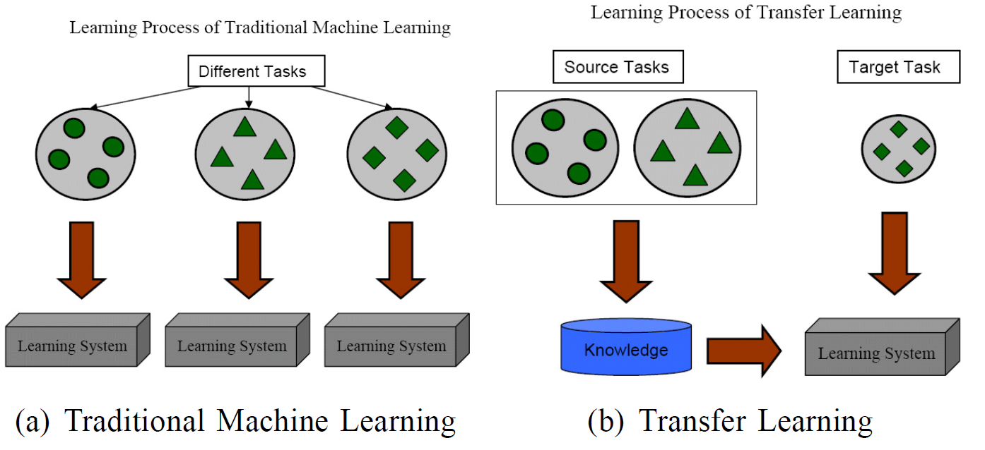
Transfer Learning vs Multi-task Learning

Transfer Learning
- extract knowledge from “SOURCE task”
- apply that knowledge to “TARGET task”
Multi-task Learning
- learning all of the “SOURCE & TARGET tasks” simultaneously

(2) Notation & Definitions

( keywords : domain, task )

Domain

Domain : \(\mathcal{D}=\{\mathcal{X}, P(X)\}\)
- 1) Feature space : \(\mathcal{X}\)
- 2) Marginal pdf : \(P(X)\)
  - \(X=\left\{x_{1}, \ldots, x_{n}\right\} \in \mathcal{X}\).
Source & Target domain
- Source domain : \(\mathcal{D}_S\)
- Target domain : \(\mathcal{D}_T\)
Source & Target data
- Source domain data : \(D_{S}=\left\{\left(x_{S_{1}}, y_{S_{1}}\right), \ldots,\left(x_{S_{n_{S}}}, y_{S_{n_{S}}}\right)\right\}\)
- Target domain data : \(D_{T}=\left\{\left(x_{T_{1}}, y_{T_{1}}\right), \ldots,\left(x_{T_{n_{T}}}, y_{T_{n_{T}}}\right)\right\}\).
- ( \(0 \leq n_{T} \ll n_{S}\) )
ex) Document Classification
- if each term is taken as binary feature ( ex. “happy” = [0,1,0,0,0,1,0,…,1] )
- \(\mathcal{X}\) : space of all term vectors
  - \(x_i\) : \(i^\text{th}\) term vector ( ex. vector of “sad” )
  - \(X\) : particular learning sample ( ex. one sample document )
- 2 domains are different =
  - case 1) \(\mathcal{X}\) may be different
  - case 2) \(P(X)\) may be different

Task

Task : \(\mathcal{T}=\{\mathcal{Y}, f(\cdot)\}\)
- 1) Label space : \(\mathcal{Y}\)
- 2) Objective predictive function : \(f(\cdot)\)
  
  ( not observed, but learned from training data )
  - training data : \(\left\{x_{i}, y_{i}\right\}\), where \(x_{i} \in X\) and \(y_{i} \in \mathcal{Y}\).
ex) Document Classification
- \(\mathcal{Y}\) = \(\left\{\text{genre 1},\text{genre 2},..,\text{genre K} \right\}\)
- \(y_i\) = \(\text{genre 5}\)

Transfer Learning

given \(\mathcal{D_S},\mathcal{D_T}\), \(\mathcal{T}_S, \mathcal{T}_T\)
transfer learning aims to help improve…
- the “learning of the target predictive function \(f(\cdot)_T\)“ in \(\mathcal{D_T}\)
by using the knowledge in \(\mathcal{D_S}\) & \(\mathcal{T}_S\),
where \(\mathcal{D}_{S} \neq \mathcal{D}_{T}\) or \(\mathcal{T}_{S} \neq \mathcal{T}_{T}\)
- case 1) \(\mathcal{D}_{S} \neq \mathcal{D}_{T}\)
  - case 1-1) \(\mathcal{X}_{S} \neq \mathcal{X}_{T}\)
    - ex) ENGLISH document & KOREAN document
  - case 1-2) \(P_{S}(X) \neq P_{T}(X)\)
    - ex) document with topic “WAR” & ~ topic “LOVE”
- case 2) \(\mathcal{T}_{S} \neq \mathcal{T}_{T}\)
  - case 2-1) \(\mathcal{Y}_{S} \neq \mathcal{Y}_{T}\)
    - ex) topic (A,B) & topic (C, D,E,F)
  - case 2-2) \(P\left(Y_{S} \mid X_{S}\right) \neq P\left(Y_{T} \mid X_{T}\right)\)
    - ex) source & target are very unbalanced in terms of user-defined classes
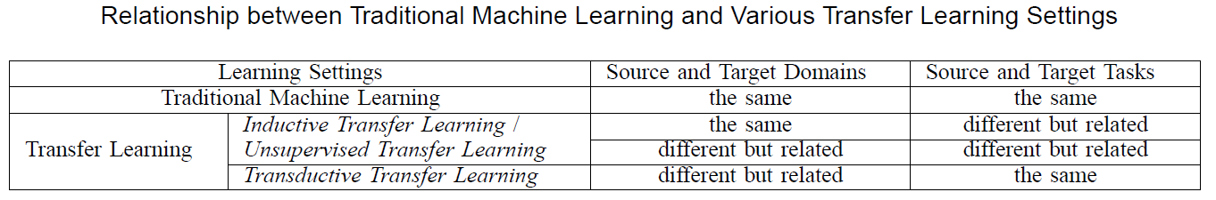
traditional ML task :
- \(\mathcal{D}_{S} = \mathcal{D}_{T}\) and \(\mathcal{T}_{S} = \mathcal{T}_{T}\)

(3) Categorization

3 main issues of TL (Transfer Learning)

1) WHAT to transfer
- which part of knowledge?
2) HOW to transfer
- algorithms to transfer knowledge
3) WHEN to transfer
- when 2 are not related, should not transfer!
  
  ( if not, “NEGATIVE TRANSFER” )

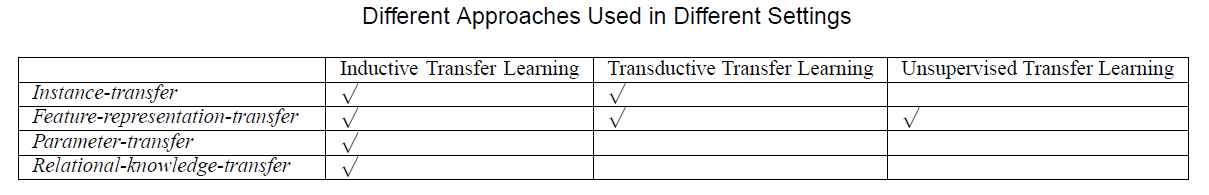
Categorization of TL

1) Inductive TL
2) Transductive TL
3) Unsupervised TL

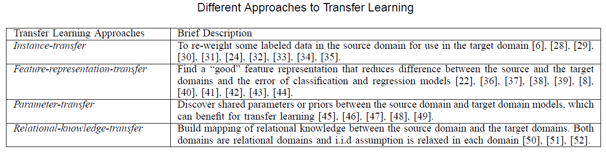
These 3 categories can be summarized into 4 cases! ( based on “WHAT to transfer” )

(1) Instance-based TL
- reuse data in source domain
- by re-weighting
  - ex) Instance re-weighting / Importance sampling
(2) Feature-representation TL
- learn a “good” feature for target domain
(3) Parameter TL
- source & target task share ‘parameters’ or ‘prior distn for hyperparameter’
(4) Relational Knowledge Transfer
- relationship among data in source & target are similar

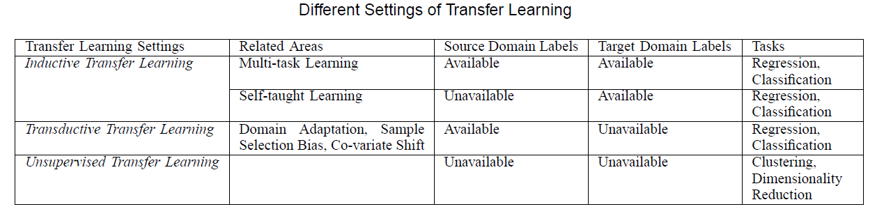
3. Inductive TL

Inductive TL : \(\mathcal{T_S} \neq \mathcal{T_T}\)

few labeled data in TARGET are required as training data to induce the target predictive function
ex) Multi-task learning
SOURCE labels : O & TARGET labels : O
ex) Self-taught learning
- SOURCE labels : X & TARGET labels : O
( more focus on MTL )

(1) Instance-based TL

idea : some SOURCE data may be RE-USED, together with few labeled TARGET data
ex) TrAdaboost

TrAdaBoost

Assumption :
- SOURCE & TARGET = same set of features & labels
- but, DISTRIBUTION of data are different
Key Idea :
- some source data may be HELPFUL
- some source data may be HARMFUL
Iteratively re-weight source domain data…
- to reduce the effect of “BAD” source data
- to encourage the effect of “GOOD” source data
to contribute more for target domain
trains the base classifier on the “weighted” source & target data

( error : calculated ONLY on TARGET data )

Jiang and Zhai

remove “misleading” training examples from source domain,

based on conditional probabilities \(P(y_T \mid x_T)\) & \(P(y_S \mid x_S)\)

(2) Feature-representation TL

idea : good feature representation to “minimize domain divergence & cls/reg error”
similar to “common feature learning” in multi-task learning
case 1) supervised
case 2) unsupervised

SUPERVISED feature construction

common features can be learned by…

\(\begin{array}{cl} \underset{A, U}{\arg \min } & \sum_{t \in\{T, S\}} \sum_{i=1}^{n_{t}} L\left(y_{t_{i}},\left\langle a_{t}, U^{T} x_{t_{i}}\right\rangle\right)+\gamma \mid \mid A \mid \mid _{2,1}^{2} \\ \text { s.t. } & U \in \mathbf{O}^{d} \end{array}\).

\(S\) & \(T\) : source & target domain
parameters : \(A=\left[a_{S}, a_{T}\right] \in R^{d \times 2}\)
mapping function : \(U\) ( \(d \times d\) orthogonal matrix )
regularization : \(\mid \mid A \mid \mid _{r, p}:=\left(\sum_{i=1}^{d}\left \mid \mid a^{i}\right \mid \mid _{r}^{p}\right)^{\frac{1}{p}}\)
Low dimension representation : \(U^{T} X_{T}, U^{T} X_{S}\)

UNSUPERVISED feature construction

ex) Sparse Coding

step 1) higher-level basis vectors \(b = \{b_1, b_2, ..., b_s\}\) are learned on SOURCE
- \(\begin{gathered} \min _{a, b} \sum_{i}\left \mid \mid x_{S_{i}}-\sum_{j} a_{S_{i}}^{j} b_{j}\right \mid \mid _{2}^{2}+\beta\left \mid \mid a_{S_{i}}\right \mid \mid _{1} \\ \text { s.t. } \quad\left \mid \mid b_{j}\right \mid \mid _{2} \leq 1, \forall j \in 1, \ldots, s \end{gathered}\).
- \(a_{S_{i}}^{j}\) : new representation ( of basis \(b_{j}\) for input \(x_{S_{i}}\) )
step 2) applied on TARGET domain, based on basis vector \(b\)
- \(a_{T_{i}}^{*}=\underset{a_{T_{i}}}{\arg \min }\left \mid \mid x_{T_{i}}-\sum_{j} a_{T_{i}}^{j} b_{j}\right \mid \mid _{2}^{2}+\beta\left \mid \mid a_{T_{i}}\right \mid \mid _{1}\).
then, use discriminative algorithm for \(\left\{a_{T_{i}}^{*}\right\}^{\prime} s\)

(3) Parameter TL

most are designed under MTL framework
difference
- MTL : all tasks are equally important
- TL : weights in loss functions for different domains can be different!

(4) Relational Knowledge Transfer

TL problems in relational domains
pass

4. Transductive TL

Transductive TL : \(\mathcal{T_S} = \mathcal{T_T}\) & \(\mathcal{D_S} \neq \mathcal{D_T}\)

only require SOME of the unlabeled TARGET data to be seen while training
meaning of transductive
- (original)
  - ALL test data be seen while tranining
  - trained model cannot be used for FUTURE data
  - when new data arrive, must re-train using ALL data
- (transductive TL)
  - “TASKS” must be same
  - must be some unlabeled data in target
also known as “DOMAIN ADAPTATION”
2 cases of \(\mathcal{D_S} \neq \mathcal{D_T}\)
- 1) \(\mathcal{X}_{S} \neq \mathcal{X}_{T}\)………….. ex) ENGLISH document & KOREAN document
- 2) \(P_{S}(X) \neq P_{T}(X)\) …. ex) document with topic “WAR” & ~ topic “LOVE”

(1) Instance-based TL

most are based on “IMPORTANCE sampling”
minimize ERM (Empirical Risk Minimization)
- \(\theta^{*}=\underset{\theta \in \Theta}{\arg \min } \frac{1}{n} \sum_{i=1}^{n}\left[l\left(x_{i}, y_{i}, \theta\right)\right]\).
In TL setting…
- if \(P\left(D_{S}\right)=P\left(D_{T}\right)\) :
  - \(\theta^{*}=\underset{\theta \in \Theta}{\arg \min } \sum_{(x, y) \in D_{S}} P\left(D_{S}\right) l(x, y, \theta) \text {. }\).
- if \(P\left(D_{S}\right) \neq P\left(D_{T}\right)\) :
  - \(\begin{aligned} \theta^{*} &=\underset{\theta \in \Theta}{\arg \min } \sum_{(x, y) \in D_{S}} \frac{P\left(D_{T}\right)}{P\left(D_{S}\right)} P\left(D_{S}\right) l(x, y, \theta) \\ & \approx \underset{\theta \in \Theta}{\arg \min } \sum_{i=1}^{n_{S}} \frac{P_{T}\left(x_{T_{i}}, y_{T_{i}}\right)}{P_{S}\left(x_{S_{i}}, y_{S_{i}}\right)} l\left(x_{S_{i}}, y_{S_{i}}, \theta\right) . \end{aligned}\).
Add different penalty values to each instance \(\left(x_{S_{i}}, y_{S_{i}}\right)\),

with the corresponding weight \(\frac{P_{T}\left(x_{T_{i}}, y_{T_{i}}\right)}{P_{S}\left(x_{S_{i}}, y_{S_{i}}\right)}=\frac{P\left(x_{T_{i}}, y_{T_{i}}\right)}{P\left(x_{S_{i}}, y_{S_{i}}\right)}\) ( since \(P(Y_T \mid X_T) = P(Y_S \mid X_S)\) )
Different ways to estimate the ratio!
- ex) KMM (Kernel-mean matching)
- ex) KLIEP (Kullback-Leibler Importance Estimation Procedure)
besides re-weighting…
- ex) extend NB classifier for “transductive transfer learning”

(2) Feature-representation TL

most are “UNsupervised” approach
SCL (Structural Correspondence Learning algorithm)
- step 1) define \(m\) pivot features ( on UNlabeled data from \(S\) & \(T\) )
- step 2) remove these pivot & treat each pivot as new label vector
- step 3) train \(m\) linear classifier
- step 4) SVD on \(W\)
- step 5) standard discriminative algorithms can be applied to “augmented feature vector” to build models
Transfer Learning in NLP => “Domain Adaptation”
- kernel-mapping function
Dimensionality Reduction
- MMDE (Maximum Mean Discrepency Embedding)
  - problem : “computational burden”
- solution : TCA (Transfer Component Analysis)

5. Unsupervised TL

pass

6. Transfer Bounds & Negative Transfer

Kolmogorov complexity

conditional Kolmogorov complexity to measure “relatedness between tasks”
transfer the “right” amount of information
under a Bayesian framework

Eaton et al

graph-based method for knowledge transfer

Learning tasks can be divided into groups

same group = share low-dim representation

Therefore, by adding different penalty values to each instance \(\left(x_{S_{i}}, y_{S_{i}}\right)\) with the corresponding weight \(\frac{P_{T}\left(x_{T_{i}}, y_{T_{i}}\right)}{P_{S}\left(x_{S_{i}}, y_{S_{i}}\right)}\), we can

Twitter Facebook LinkedIn

(paper) A Survey on Transfer Learning

A Survey on Transfer Learning

Seunghan Lee

A Survey on Transfer Learning

Contents

0. Abstract

1. Introduction

2. Overview

(1) Brief History

(2) Notation & Definitions

Domain

Task

Transfer Learning

(3) Categorization

3. Inductive TL

(1) Instance-based TL

TrAdaBoost

Jiang and Zhai

(2) Feature-representation TL

SUPERVISED feature construction

UNSUPERVISED feature construction

(3) Parameter TL

(4) Relational Knowledge Transfer

4. Transductive TL

(1) Instance-based TL

(2) Feature-representation TL

5. Unsupervised TL

6. Transfer Bounds & Negative Transfer

You May Also Enjoy