[Paper Review] 30.Few-shot Image Generation via Cross-domain Correspondence

[Paper Review] 30. Few-shot Image Generation via Cross-domain

Contents

1. Abstract
2. Introduction
3. Related Works
4. Approach
   1. Cross-domain distance consistencey
   2. Relaxed realism with few examples
   3. Final Objective

0. Abstract

limited # of target domain samples \(\rightarrow\) overfitting

how to solve?

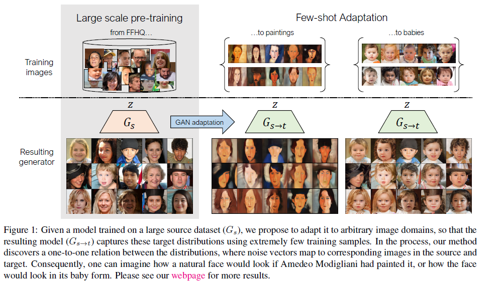
• utilize a large source domain for pretraining
• transfer the diversity information from “source to target”

key point : preserve relation(sim/dissim) between source instances

Proposes…

• 1) cross-domain distance consistency loss
• 2) anchor-based strategy

1. Introduction

Transfer Learning

• key idea : source -> target domain
• BUT…. need more than 100 training images

This paper : explore transferring different kind of info from source!

• how images relate to each other !

  ( preserve relation (similarity & difference) in source domain)

• introduce cross-domain distance consistency loss

  • enforce similarity before & after adaptation

enforce realism in 2 different ways

• 1) image-level adversarial loss,

  on synthesized images, which should map to one of the real samples

• 2) patch-level adversarial loss,

  for all other synthesized images

Contribution

enforce cross-domain correspondence for few-shot image generation

2. Related Work

1) Few shot learning

Few-shot image generation :

• make new & diverse images, while preventing overfitting to few samples

This paper : regularize adaptation by…

transferring “how image relate to each other in source domain “ to target domain

2) Domain Translation

• translate image from source to target

3) Distance preservation

To alleviate mode collapse…..

DistanceGAN :

• proposes to preserve the distances between input pairs

This paper :

• inherit learned diversity from source model to target model
• by using cross-domain distance consistency loss

3. Approach

Notation

• \(G_{s}\) : source generator
  • mapping : \(z \rightarrow x\)
• \(\mathcal{D}_{s}\) : source dataset ( LARGE )
• \(D_t\) : target dataset ( SMALL )

Goal

• learn an adapted generator \(G_{s \rightarrow t}\)
• how?
  • 1) initialize \(\theta\) to the source generator
  • 2) fitting it to \(D_t\)

Objective function

• \(\mathcal{L}_{\text {adv }}(G, D)=D(G(z))-D(x)\).

• \(G_{s \rightarrow t}^{*}=\mathbb{E}_{z \sim p_{z}(z), x \sim \mathcal{D}_{t}} \arg \min _{G} \max _{D} \mathcal{L}_{\text {adv }}(G, D)\).

BUT overfits in few-dataset….. then HOW?

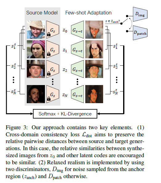
propose a cross-domain consistency loss!

3-1) Cross-domain distance

consequence of overfitting

• relative distances in the source domain is NOT PRESERVED

Thus, by enforcing preservation of distances \(\rightarrow\) help prevent collapse!

pdf of \(i\)th noise vector for…

• source generator

  • \[y_{i}^{s, l} =\operatorname{Softmax}\left(\left\{\sin \left(G_{s}^{l}\left(z_{i}\right), G_{s}^{l}\left(z_{j}\right)\right)\right\}_{\forall i \neq j}\right)\]

• adapted generator

  • \(y_{i}^{s \rightarrow t, l} =\operatorname{Softmax}\left(\left\{\operatorname{sim}\left(G_{s \rightarrow t}^{l}\left(z_{i}\right), G_{s \rightarrow t}^{l}\left(z_{j}\right)\right)\right\}_{\forall i \neq j}\right)\).

  ( sim = cosine similarity )

inspired by contrastive learning…

• encourage adapted model to be similar to that of source
• \(\mathcal{L}_{\text {dist }}\left(G_{s \rightarrow t}, G_{s}\right)=\mathbb{E}_{\left\{z_{i} \sim p_{z}(z)\right\}} \sum_{l, i} D_{K L}\left(y_{i}^{s \rightarrow t, l} \| y_{i}^{s, l}\right) .\).

3-2) Relaxed realism with few examples

Enforce adversarial loss, using a path-level discriminator (\(D_{\text {patch }}\))

• \(\mathcal{L}_{\text {adv }}^{\prime}\left(G, D_{\text {img }}, D_{\text {patch }}\right)=\mathbb{E}_{x \sim \mathcal{D}_{t}} \left[\mathbb{E}_{z \sim Z_{\text {anch }}} \mathcal{L}_{\text {adv }}\left(G, D_{\text {img }}\right)\right. \left.+\mathbb{E}_{z \sim p_{z}(z)} \mathcal{L}_{\text {adv }}\left(G, D_{\text {patch }}\right)\right]\).

3-3) Final Objective

\(G_{s \rightarrow t}^{*}=\arg \min _{G} \max _{D_{\text {img }}, D_{\text {pach }}} \mathcal{L}_{\text {adv }}^{\prime}\left(G, D_{\text {img }}, D_{\text {patch }}\right) +\lambda \mathcal{L}_{\text {dist }}\left(G, G_{s}\right)\).

2 terms :

• 1) \(\mathcal{L}^{\prime}\) : deals with appearance of target
• 2) \(\mathcal{L}_{\text {dist }}\) : to preserve structural diversity