
Diffusion Models for Tabular Data Imputation and Synthetic Data Generation
Contents
-
Abstract
0. Abstract
Use of diffusion models with transformer conditioning for both
- (1) data imputation
- (2) data generation
Transformer conditioning
- harness the ability of transformers to model dependencies and cross-feature interactions within tabular data.
1. Introduction
Consider synthetic data generation as a general case of data imputation
TabGenDDPM
- New conditioning in diffusion model for tabular data using a transformer
- Special masking mechanism
- makes it possible to tackle both tasks with a single model
Contributions
- (1) Incorporation of a transformer within the diffusion model
- to model inter-feature interactions better within tabular data.
- (2) Innovative masking & conditioning strategy on features
- enabling both data imputation and generation with a single model.
- (3) SOTA in Machine Learning (ML) utility and statistical similariy
2. Related Work
(1) Diffusion Models
Pass
(2) Data Imputation
Traditional approaches
- ex) Involve removing rows or columns with missing entries
- ex) Filling gaps with average values for a particular feature.
Recent trends
- ML techniques
- Deep generative models
(3) Generative Models
Generative models for tabular data
- Tabular VAEs and GANs
- ex) TabDDPM
- powerful method for tabular data generation, leveraging the strengths of Diffusion Models.
$\rightarrow$ TabGenDDPM builds upon TabDDPM, targeting both tabular data generation and imputation.
3. Background
(1) Diffusion
Forward process
- $q\left(x_{1: T} \mid x_0\right)=\prod_{t=1}^T q\left(x_t \mid x_{t-1}\right)$ .
Reverse process
- $p\left(x_{0: T}\right)=\prod_{t=1}^T p\left(x_{t-1} \mid x_t\right)$.
Loss function: variational lower bound
- $L_{\mathrm{vlb}} :=L_0+L_1+\ldots+L_{T-1}+L_T $.
- $L_0 :=-\log p_\theta\left(x_0 \mid x_1\right)$.
- $L_{t-1} :=D_{K L}\left(q\left(x_{t-1} \mid x_t, x_0\right) | p_\theta\left(x_{t-1} \mid x_t\right)\right)$.
- $L_{t-1} :=D_{K L}\left(q\left(x_{t-1} \mid x_t, x_0\right) | p_\theta\left(x_{t-1} \mid x_t\right)\right)$.
- $L_T :=D_{K L}\left(q\left(x_T \mid x_0\right) | p\left(x_T\right)\right)$.
a) Gaussian diffusion models
Operate in continuous spaces $\left(x_t \in \mathbb{R}^n\right)$
Forward process
- $q\left(x_t \mid x_{t-1}\right):=\mathcal{N}\left(x_t ; \sqrt{1-\beta_t} x_{t-1}, \beta_t I\right)$.
- where $\pi=\left[\alpha_t x_t+\left(1-\alpha_t\right) / C l\right] \odot\left[\bar{\alpha}{t-1} x_0+\left(1-\bar{\alpha}{t-1}\right) / C l\right]$.
Prior
- $q\left(x_T\right):=\mathcal{N}\left(x_T ; 0, I\right)$.
Reverse process
- $p_\theta\left(x_{t-1} \mid x_t\right):=\mathcal{N}\left(x_{t-1} ; \mu_\theta\left(x_t, t\right), \Sigma_\theta\left(x_t, t\right)\right)$.
Noise prediction
- $\mu_\theta\left(x_t, t\right)=\frac{1}{\sqrt{\alpha_t}}\left(x_t-\frac{\beta_t}{\sqrt{1-\bar{\alpha}t}} \epsilon\theta\left(x_t, t\right)\right)$.
Loss
- $\mu_\theta\left(x_t, t\right)=\frac{1}{\sqrt{\alpha_t}}\left(x_t-\frac{\beta_t}{\sqrt{1-\bar{\alpha}t}} \epsilon\theta\left(x_t, t\right)\right)$.
b) Multinomial diffusion models
Generate categorical data where $x_t \in{0,1}^{C l}$ is a one-hot encoded categorical variable with $C l$ classes.
Forward process
- $q\left(x_t \mid x_{t-1}\right):=\operatorname{Cat}\left(x_t ;\left(1-\beta_t\right) x_{t-1}+\beta_t / C l\right)$.
- $q\left(x_t \mid x_0\right):=\operatorname{Cat}\left(x_t ; \bar{\alpha}_t x_0+\left(1-\bar{\alpha}_t\right) / C l\right)$.
Prior
- $q\left(x_T\right):=\operatorname{Cat}\left(x_T ; 1 / C l\right) $.
Forward posterior
- $q\left(x_{t-1} \mid x_t, x_0\right)=\operatorname{Cat}\left(x_{t-1} ; \pi / \sum_{k=1}^{C l} \pi_k\right)$.
Reverse distribution
- $p_\theta\left(x_{t-1} \mid x_t\right)$ is parameterized as $q\left(x_{t-1} \mid x_t, \hat{x}_0\left(x_t, t\right)\right)$,
4., TabGenDDPM
Builds upon the principles of TabDDPM
- Improve its capabilities in data imputation and synthetic data generation
Key distinctions
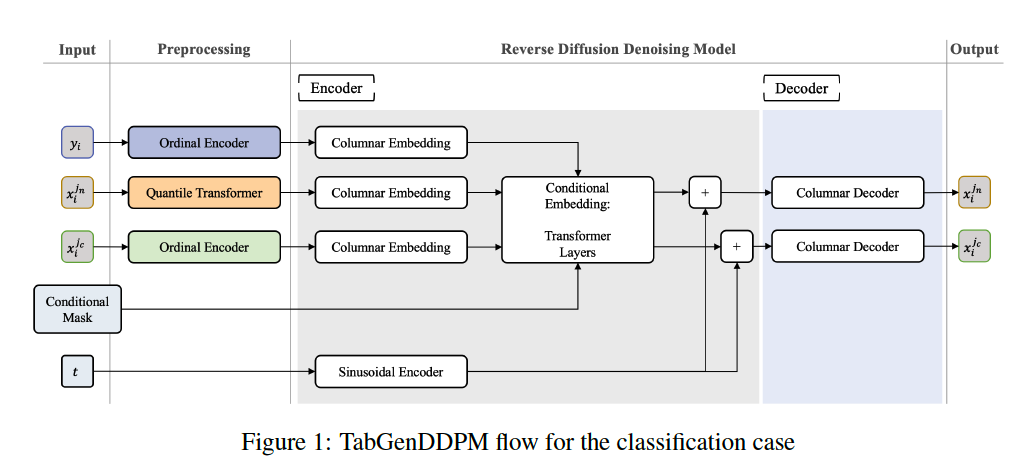
- (1) Denoising model
- [TabDDPM] a simple MLP architecture
- [TabGenDDPM] : an encoder-decoder structure
- columnar embedding and transformer architecture
- Boost synthetic data quality & offer improved conditioning for the reverse diffusion process
- (2) Conditioning mechanism.
(1) Problem Definition
- $D=\left{x_i^{j_c}, x_i^{j_n}, y_i\right}_{i=1}^N$ ,
- $x_i^{j_n}$ with $j_n \in$ $\left[1, K_{\text {num }}\right]$ : set of numerical features,
- $x_i^{j_c}$ with $j_c \in\left[1, K_{c a t}\right]$ : set of categorical features, $y_i$ is the label
- $i \in[1, N]$ : dataset rows
- $N$ : total number of rows
- $K=K_{\text {num }}+K_{\text {cat }}$ : total number of features.
Consistent preprocessing procedure across our benchmark datasets
- [Numerical] Gaussian quantile transformation
-
[Categorical] Ordinal encoding
- Missing values are replaced with zeros
Modeling
- [Numerical] with Gaussian diffusion
- [Categorical] with multinomial diffusion
TabGenDDPM
- generalizes the approach of TabDDPM
- [TabDDPM] learns $p\left(x_{t-1} \mid x_t, y\right)$,
- [TabGenDDPM] extend this by …
- allowing conditioning on a target variable $y$ and a subset of input features
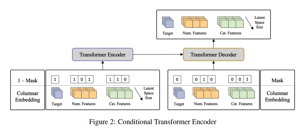
(Details) Partition variable $x$ into $x^M$ and $\bar{x}^M$.
- $x^M$ : Masked variables set
- perturbed by the forward diffusion process
- $\bar{x}^M$ : Untouched variable subset
- conditions the reverse diffusion.
$\rightarrow$ Models $p\left(x_{t-1}^M \mid x_t^M, \bar{x}^M, y\right)$, with $\bar{x}^M$ remaining constant across timesteps $t$.
Results
- enhances model performance in data generation
- enables the possibility of performing data imputation with the same model.
Reverse diffusion process $p\left(x_{t-1}^M \mid x_t^M, \bar{x}^M, y\right)$
- [Numerical] estimate the amount of noise added
- [Categorical] predict the (logit of) distribution of the categorical variable a $t=0$.
Output dim = $K_{n u m}+\sum_{i=1}^{K_{c a t}} C l_i$
- where $C l_i$ is the number of classes of $i$-th categorical feature