CoDi; Co-evolving Contrastive Diffusion Models for Mixed-type Tabular Synthesis

CoDi: Co-evolving Contrastive Diffusion Models for Mixed-type Tabular Synthesis

Contents

1. Abstract

2. Introduction

3. Background

4. Proposed Method

   1. Co-evovling Conditional Diffusion Models
   2. Contrastive Learning
   3. Training & Sampling

0. Abstract

Difficulty in modeling discrete variables of tabular data

\(\rightarrow\) Propose CoDi

CoDi

• Process continuous and discrete variables separately
  • but being conditioned on each other
  • by two diffusion models
• Two diffusion models are co-evolved
  • by reading conditions from each other
• Introduce a contrastive learning method with a negative sampling

1. Introduction

Challenging issue in the SOTA tabular data synthesis methods

\(\rightarrow\) usually consists of mixed data types

\(\rightarrow\) pre/postprocessing of the tabular data is inevitable

( & performance is highly dependent on the pre/post-processing method )

The most common way (to treat discrete variables)

= sample in “continuous spaces” after their one-hot encoding

Problems?

• (1) May lead to sub-optimal results due to sampling mistakes.
• (2) When continuous and discrete variables are processed in a same manner, it is likely that inter-column correlations are compromised in the learned distribution.

\(\rightarrow \therefore\) Interested in processing continuous and discrete variables in more robust ways

CoDi

• Incorporates two diffusion models
  • (1) For continuous variables
    • works in a continuous space
  • (2) For categorical variables
    • works in a discrete space
• Two design points
  • (1) co-evolving conditional diffusion models
  • (2) contrastive training for better connecting them

Notation

• \(\mathbf{x}_0=\left(\mathbf{x}_0^C, \mathbf{x}_0^D\right)\), which consists of continuous and discrete values
• \(\mathbf{x}_t=\left(\mathbf{x}_t^C, \mathbf{x}_t^D\right)\) : diffused sample at step \(t\).

a) Co-evolving conditional diffusion models

Read conditions from each other

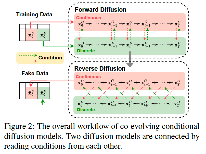
[Forward]

• Simultaneously perturb continuous and discrete variables at each forward step
  • Continuous (resp. discrete) model reads the perturbed discrete (resp. continuous) sample as a condition at the same time step.

[Reverse]

• Model denoises the sample \(\mathrm{x}_t^C\) (resp. \(\mathbf{x}_t^D\) ) conditioned both on the continuous sample \(\mathbf{x}_{t+1}^C\) and discrete sample \(\mathbf{x}_{t+1}^D\) from its previous step.

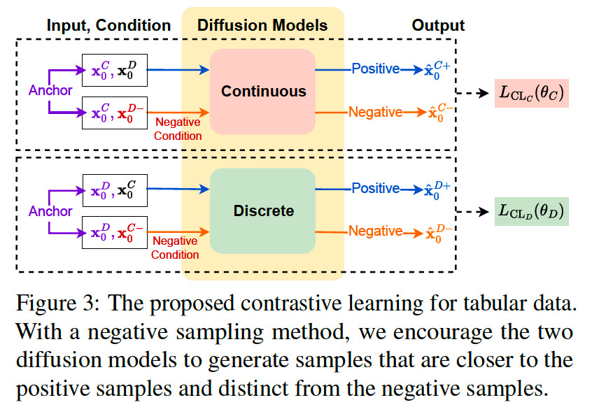
b) Contrastive learning for tabular data

• CL : Applied to the continuous and discrete diffusion models separately

• Negative sampling method for tabular data

  • focuses on defining a negative condition that permutes the pair of continuous and discrete variable sets.

Procedures (ex. conditional diffusion model)

• From anchor sample \(\mathbf{x}_0^C\),
• [POS] Generate a continuous positive sample \(\hat{\mathbf{x}}_0^{C+}\)
  • from a continuous diffusion model
  • conditioned on \(\mathbf{x}_0^D\).
• [NEG] For a negative sample \(\hat{\mathbf{x}}_0^{C-}\),
  • we randomly permute the condition parts
  • negative condition \(\mathrm{x}_0^{D-}\) is an inappropriate counterpart for \(\mathbf{x}_0^C\).

2. Background

(1) Diffusion

Forward

• \(q\left(\mathbf{x}_{1: T} \mid \mathbf{x}_0\right):=\prod_{t=1}^T q\left(\mathbf{x}_t \mid \mathbf{x}_{t-1}\right)\).

Backward

• \(p_\theta\left(\mathbf{x}_{0: T}\right):=p\left(\mathbf{x}_T\right) \prod_{t=1}^T p_\theta\left(\mathbf{x}_{t-1} \mid \mathbf{x}_t\right)\).

a) Continuous space

Prior distribution \(p\left(\mathbf{x}_T\right)=\mathcal{N}\left(\mathbf{x}_T ; \mathbf{0}, \mathbf{I}\right)\),

Forward

• \(q\left(\mathbf{x}_t \mid \mathbf{x}_{t-1}\right)=\mathcal{N}\left(\mathbf{x}_t ; \sqrt{1-\beta_t} \mathbf{x}_{t-1}, \beta_t \mathbf{I}\right)\).

Backward

• \(p_\theta\left(\mathbf{x}_{t-1} \mid \mathbf{x}_t\right)=\mathcal{N}\left(\mathbf{x}_{t-1} ; \boldsymbol{\mu}_\theta\left(\mathbf{x}_t, t\right), \mathbf{\Sigma}_\theta\left(\mathbf{x}_t, t\right)\right)\).

Loss function

• \(L_{\text {simple }}(\theta):=\mathbb{E}_{t, \mathbf{x}_0, \boldsymbol{\epsilon}}\left[ \mid \mid \boldsymbol{\epsilon}-\boldsymbol{\epsilon}_\theta\left(\mathbf{x}_t, t\right) \mid \mid ^2\right]\).

b) Discrete space

The diffusion process can be defined in discrete spaces using categorical distributions.

Forward

• \(q\left(\mathbf{x}_t \mid \mathbf{x}_{t-1}\right) =\mathcal{C}\left(\mathbf{x}_t ;\left(1-\beta_t\right) \mathbf{x}_{t-1}+\beta_t / K\right)\).

Backward

• \(p_\theta\left(\mathbf{x}_{t-1} \mid \mathbf{x}_t\right) =\sum_{\hat{\mathbf{x}}_0=1}^K q\left(\mathbf{x}_{t-1} \mid \mathbf{x}_t, \hat{\mathbf{x}}_0\right) p_\theta\left(\hat{\mathbf{x}}_0 \mid \mathbf{x}_t\right)\).
  • where \(\mathcal{C}\) indicates a categorical distribution
  • \(K\) is the number of categories
  • uniform noise is added

(2) Tabular Data Synthesis

pass

3. Proposed Method

(1) Co-evolving Conditional Diffusion Models

Given a sample \(\mathbf{x}_0\) , where \(\mathbf{x}_0=\left(\mathbf{x}_0^C, \mathbf{x}_0^D\right)\).

• \(N_C\) continuous columns \(C=\left\{C_1, C_2, \ldots, C_{N_C}\right\}\)
• \(N_D\) discrete columns \(D=\) \(\left\{D_1, D_2, \ldots, D_{N_D}\right\}\),

Two diffusion models read conditions from each other

• continuous and discrete diffusion models

To generate one related data pair with two models, we input each other’s output as a condition

Pair \(\left(\mathbf{x}_0^C, \mathbf{x}_0^D\right)\) are then simultaneously perturbed at each forward time step

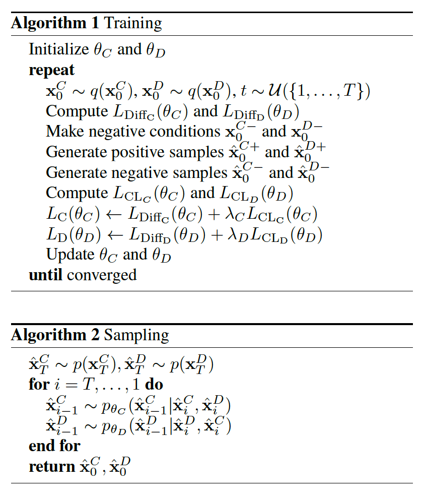
Parameter \(\theta_C\) (resp. \(\theta_D\) ) is updated based on …

• \(L_{\mathrm{Diff}_{\mathrm{C}}}\left(\theta_C\right):=\mathbb{E}_{t, \mathbf{x}_0^C, \boldsymbol{\epsilon}}\left[ \mid \mid \boldsymbol{\epsilon}-\boldsymbol{\epsilon}_{\theta_C}\left(\mathbf{x}_t^C, t \mid \mathbf{x}_t^D\right) \mid \mid ^2\right]\).
• \(L_{\text {Diff }_{\mathrm{D}}}\left(\theta_D\right)= \mathbb{E}_q[\underbrace{D_{\mathrm{KL}}\left[q\left(\mathbf{x}_T^D \mid \mathbf{x}_0^D\right) \mid \mid p\left(\mathbf{x}_T^D\right)\right]}_{L_T} \underbrace{-\log p_{\theta_D}\left(\mathbf{x}_0^D \mid \mathbf{x}_1^D, \mathbf{x}_1^C\right)}_{L_0}+\sum_{t=2}^T \underbrace{D_{\mathrm{KL}}\left(q\left(\mathbf{x}_{t-1}^D \mid \mathbf{x}_t^D, \mathbf{x}_0^D\right) \mid \mid p_{\theta_D}\left(\mathbf{x}_{t-1}^D \mid \mathbf{x}_t^D, \mathbf{x}_t^C\right)\right)}_{L_{t-1}}]\).

[ Reverse Process ]

• Generated samples, \(\hat{\mathbf{x}}_0^C\) and \(\hat{\mathbf{x}}_0^D\), are progressively synthesized from each noise space.
• The prior distributions
  • \(p\left(\mathbf{x}_T^C\right)=\mathcal{N}\left(\mathbf{x}_T^C ; \mathbf{0}, \mathbf{I}\right)\) .
  • \(p\left(\mathbf{x}_T^{D_i}\right)=\mathcal{C}\left(\mathbf{x}_T^{D_i} ; 1 / K_i\right)\),
    • where \(\left\{K_i\right\}_{i=1}^{N_D}\) is the number of categories of the discrete column \(\left\{D_i\right\}_{i=1}^{N_D}\).

a) Forward

\(\begin{array}{r} q\left(\mathbf{x}_t^C \mid \mathbf{x}_0^C\right)=\mathcal{N}\left(\mathbf{x}_t^C ; \sqrt{\bar{\alpha}_t} \mathbf{x}_0^C,\left(1-\bar{\alpha}_t\right) \mathbf{I}\right), \\ q\left(\mathbf{x}_t^{D_i} \mid \mathbf{x}_0^{D_i}\right)=\mathcal{C}\left(\mathbf{x}_t^{D_i} ; \bar{\alpha}_t \mathbf{x}_0^{D_i}+\left(1-\bar{\alpha}_t\right) / K_i\right), \end{array}\).

• where \(1 \leq i \leq N_D, \alpha_t:=1-\beta_t\) and \(\bar{\alpha}_t:=\prod_{i=1}^t \alpha_i\).

b) Reverse

\(\begin{gathered} p_{\theta_C}\left(\mathbf{x}_{0: T}^C\right):=p\left(\mathbf{x}_T^C\right) \prod_{t=1}^T p_{\theta_C}\left(\mathbf{x}_{t-1}^C \mid \mathbf{x}_t^C, \mathbf{x}_t^D\right), \\ p_{\theta_D}\left(\mathbf{x}_{0: T}^{D_i}\right):=p\left(\mathbf{x}_T^{D_i}\right) \prod_{t=1}^T p_{\theta_D}\left(\mathbf{x}_{t-1}^{D_i} \mid \mathbf{x}_t^{D_i}, \mathbf{x}_t^C\right), \end{gathered}\).

• where \(1 \leq i \leq N_D\) and the reverse transition probabilities

(2) Contrastive Learning

Triplet Loss

• \(L_{\mathrm{CL}}(A, P, N)=\sum_{i=0}^S\left[\max \left\{d\left(A_i, P_i\right)-d\left(A_i, N_i\right)+m, 0\right\}\right]\).

Final Loss function

• \(L_{\mathrm{C}}\left(\theta_C\right)=L_{\text {Diff }_{\mathrm{C}}}\left(\theta_C\right)+\lambda_C L_{\mathrm{CL}}\left(\theta_C\right)\).

• \(L_{\mathrm{D}}\left(\theta_D\right)=L_{\text {Diff }_D}\left(\theta_D\right)+\lambda_D L_{\mathrm{CL}_{\mathrm{D}}}\left(\theta_D\right)\).

Negative Condition

• Negative conditions, \(\mathbf{x}_0^{D-}\) and \(\mathbf{x}_0^{C-}\), are the keys to generate the negative samples
• By randomly shuffling the continuous and discrete variable sets so that they do not match

(3) Training & Sampling