Hierarchical Softmax

Hierarchical Softmax

( 참고 : word2vec Parameter Learning Explained ( Xin Rong, 2016 ))

WHY hierarchical softmax?

• “binary tree를 사용하여 softmax를 효율적으로 연산하는 방법”

• 기존의 softmax보다 빠르게 연산할 수 있음

• NLP에서 자주 사용

  ( 수 많은 word들! output의 개수가 다른 기타 분류문제보다, 훨씬 많아서 기존의 방법으로는 너무 많은 연산량을 필요로 한다 )

Introduction

Tree 방식을 이용하여 연산이 이루어진다. V개의 단어가 tree의 leaf node가 되고, 각각의 leaf unit에는 root unit까지 가는 unique path가 있다. leaf unit의 이러한 path는 해당 leaf unit(단어)가 나올 확률을 계산하는 데에 있어서 이용된다.
아래 그림은 hierarchical softmax의 구조를 보여준다

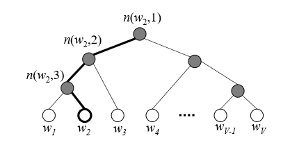
최하단의 하얀 leaf node(\(w_1\)~\(w_V\))는 각각 \(V\)개의 단어를 나타내고, 어둡게 칠해진 부분은 inner unit이다(\(V-1\)개). 굵게 칠해진 path는 단어 \(w_2\)가 root까지 가는 path를 보여준다. 이 path의 길이는 \(L(w_2)=4\)이다. \(n(w,j)\)는 root unit에서 단어 \(w\)까지 가는 path에 있는 \(j\)번째 unit을 나타낸다.

[Huffman Tree] Tree에서 각각의 leaf에 word들을 배치할때, 임의로 하는 대신에, deep level에는 빈도수가 적은 단어를, low level에는 빈도수가 많은 단어를 할당하는 방식을 뜻한다.

Algorithm

hierarchical softmax는 기존의 softmax와 다르게, 출력으로써 leaf unit(단어)에 대한 vector representation이 없다. 대신, \(V-1\)개의 inner unit는 output vector \(\mathbf{v}'_{n(w,j)}\)를 가지고, 각 단어가 output word가 될 확률은 다음과 같이 계산된다.

\(p\left(w=w_{O}\right)=\prod_{j=1}^{L(w)-1} \sigma\left(\ll n(w, j+1)=\operatorname{ch}(n(w, j)) \gg \cdot \mathbf{v}_{n(w, j)}^{\prime} \mathbf{h}\right)\).

• \(\operatorname{ch}(n)\) : unit n의 왼쪽 child node

• \(\mathbf{v}'_{n(w,j)}\) : inner unit \(n(w,j)\)의 vector representation(output vector)

• \(\mathbf{h}\) : hidden layer의 output vector

  ( input으로 들어가는 word의 vector이다.

  Skip-Gram의 경우에는 중심 단어의 vector, CBOW의 경우 그 주변의 context 단어들의 평균 vector )

• \(\ll x \gg=\left\{\begin{array}{ll} 1 & \text { if } x \text { is true } \\ -1 & \text { otherwise } \end{array}\right.\).

복잡해보이는 해당 수식을 직관적으로 생각해보자.

위 그림의 예시로 표현하자면, 우리는 \(w_2\)가 output으로 나올 확률을 구하는 과정은 root 부터 시작해서 \(w_2\)에 도달할 random walk의 확률로 볼 수 있다. 그 path를 지나면서 거치는 각각의 inner unit에서, 우리는 왼쪽으로 갈지 오른쪽으로 갈지에 대한 확률을 계산할 필요가 있다. inner unit n에서 왼쪽으로 갈 확률을 다음과 같이 정의한다.

\(p(n, \text { left })=\sigma\left(\mathrm{v}_{n}^{\prime T} \cdot \mathrm{h}\right)\).

위 식을 보면 알 수 있듯, inner unit이 어느 방향으로 갈 지는 inner unit의 output vector과 hidden layer의 output value에 의해 결정된다. 반대로, inner unit에서 오른쪽으로 갈 확률은 다음과 같이 표현될 수 있다.

\(p(n, \text { right })=1-\sigma\left(\mathbf{v}_{n}^{\prime T} \cdot \mathbf{h}\right)=\sigma\left(-\mathbf{v}_{n}^{\prime T} \cdot \mathbf{h}\right)\).

이를 토대로, 위 그림에서 \(w_2\)가 나올 확률을 계산하면 다음과 같다.

\(\begin{aligned} p\left(w_{2}=w_{O}\right) &=p\left(n\left(w_{2}, 1\right), \text { left }\right) \cdot p\left(n\left(w_{2}, 2\right), \text { left }\right) \cdot p\left(n\left(w_{2}, 3\right), \text { right }\right) \\ &=\sigma\left(\mathbf{v}_{n\left(w_{2}, 1\right)}^{\prime} \mathbf{h}\right) \cdot \sigma\left(\mathbf{v}_{n\left(w_{2}, 2\right)}^{\prime} \mathbf{h}\right) \cdot \sigma\left(-\mathbf{v}_{n\left(w_{2}, 3\right)}^{\prime} \mathbf{h}\right) \end{aligned}\).

다음과 같은 특징은 hierarchical softmax가 단어들의 multinomial distribution으로 정의할 수 있음을 보여준다.

\(\sum_{i=1}^{V} p\left(w_{i}=w_{O}\right)=1\).

Updating Equation

간단한 이해를 위해 one-word context모델로 설명을 한다. 이를 CBOW나 skip-gram 모델로 확장하는 것은 쉽다.

우선 간단한 표현을 위해, 다음과 같이 축약해서 표현한다

\(\ll \cdot \gg :=\ll n(w, j+1)=\operatorname{ch}(n(w, j)) \gg\).

\(\mathbf{v}_{j}^{\prime}:=\mathbf{v}_{n_{w, j}}^{\prime}\).

Error function은 아래와 같이 정의된다.

\(E=-\log p\left(w=w_{O} \mid w_{I}\right)=-\sum_{j=1}^{L(w)-1} \log \sigma\left(\ll \cdot \gg \mathbf{v}_{j}^{\prime T} \mathbf{h}\right)\).

이 E를 에 대해 미분하면,

\(\begin{aligned} \frac{\partial E}{\partial \mathbf{v}_{j}^{\prime} \mathbf{h}} &=\left(\sigma\left(\ll \cdot \gg \mathbf{v}_{j}^{\prime T} \mathbf{h}\right)-1\right) \ll \cdot \gg \\ &=\left\{\begin{array}{ll} \sigma\left(\mathbf{v}_{j}^{\prime T} \mathbf{h}\right)-1 & (\ll \cdot \gg=1) \\ \sigma\left(\mathbf{v}_{j}^{\prime T} \mathbf{h}\right) & (\ll \cdot \gg=-1) \end{array}\right.\\ &=\sigma\left(\mathbf{v}_{j}^{\prime T} \mathbf{h}\right)-t_{j} \end{aligned}\).

where \(t_{j}=1\) if \(\ll \cdot \gg=1\) and \(t_{j}=0\) otherwise

그 다음, E를 inner unit \(n(w,j)\)로 미분하면, 우리는 chain rule에 의해 다음과 같은 결과를 얻게 된다.

\(\frac{\partial E}{\partial \mathrm{v}_{j}^{\prime}}=\frac{\partial E}{\partial \mathrm{v}_{j}^{\prime} \mathrm{h}} \cdot \frac{\partial \mathrm{v}_{j}^{\prime} \mathrm{h}}{\partial \mathrm{v}_{j}^{\prime}}=\left(\sigma\left(\mathrm{v}_{j}^{\prime T} \mathrm{~h}\right)-t_{j}\right) \cdot \mathrm{h}\).

그러므로, output vector의 updating equation은 다음과 같이 나타낼 수 있다.

\(\mathbf{v}_{j}^{\prime(\text { new })}=\mathbf{v}_{j}^{\prime(\text { old })}-\eta\left(\sigma\left(\mathbf{v}_{j}^{\prime T} \mathbf{h}\right)-t_{j}\right) \cdot \mathbf{h}\).

where \(j=1,2,....L(w)-1)\)

정리하자면, 각각의 inner unit에게 부여된 task는 해당 unit에서 왼쪽으로 갈 지, 오른쪽으로 갈 지 predict하는 문제라고 할 수 있다. 그리고, 위 식에서 \(\sigma\left(\mathbf{v}_{j}^{\prime T} \mathbf{h}\right)-t_{j}\) 는 inner unit \(n(w,j)\)의 prediction error라고 할 수 있다. 그래서 이 값이 크면(오차가 크면), 큰 폭으로 update가 이루어지고, 그 반대의 경우 update가 작게 일어나는 것을 확인할 수 있다. 이 updating equation은 CBOW와 skip-gram 모델에서 사용될 수 있다. 이것을 skip-gram 모델에서 사용한다면, 이 update 과정을 모든 C개의 단어에 대해 진행하게 되는 것이다. (skip-gram 모델은 하나의 word로 그 주변의 context word를 예측하는 모델이다) 이러한 모델들에서 weight를 update하기 위해 backpropagate하는 식은 다음과 같이 정리될 수 있다.

\(\begin{aligned} \frac{\partial E}{\partial \mathbf{h}} &=\sum_{j=1}^{L(w)-1} \frac{\partial E}{\partial \mathbf{v}_{j}^{\prime} \mathbf{h}} \cdot \frac{\partial \mathbf{v}_{j}^{\prime} \mathbf{h}}{\partial \mathbf{h}} \\ &=\sum_{j=1}^{L(w)-1}\left(\sigma\left(\mathbf{v}_{j}^{\prime T} \mathbf{h}\right)-t_{j}\right) \cdot \mathbf{v}_{j}^{\prime} \\ &:=\mathrm{EH} \end{aligned}\).

따라서, 이러한 hierarchical softmax를 통해 parameter 수를 비슷하게 유지하면서도 weight를 update하는 데에 있어서 그 연산량을 O(V)에서 O(log(V))로 획기적으로 줄일 수 있다!(ex. 1024개의 단어, binary Tree를 만들면 tree depth가 10인 Tree 생성! 연산량이 O(1024)에서 O(10)( =O(log(1024)) )로 줄어들게 됨!