(PyG) 3. GAT

Chapter 3. GAT

( 참고 : https://www.youtube.com/watch?v=JtDgmmQ60x8&list=PLGMXrbDNfqTzqxB1IGgimuhtfAhGd8lHF )

1) GAT 요약

Input & Output

• Input : OLD node feature ( \(\mathbf{h}=\left\{\bar{h}_{1}, \bar{h}_{2}, \ldots, \bar{h}_{n}\right\} \quad \bar{h}_{i} \in \mathbf{R}^{F}\) )

• Output : NEW node feature ( \(\mathbf{h}^{\prime}=\left\}_{1},{\overline{h^{\prime}}}_{2}, \ldots,{\overline{h^{\prime}}}_{n}\right\} \quad{\overline{h^{\prime}}}_{i} \in \mathbf{R}^{F^{\prime}}\) )

Attention이 이루어지는 과정

• step 1) apply parameterized LINEAR TRANSFORMATION to EVERY node
  • \(\mathbf{W} \cdot \bar{h}_{i}\) , where \(\mathbf{W} \in \mathbf{R}^{F^{\prime} \times F}\).
    

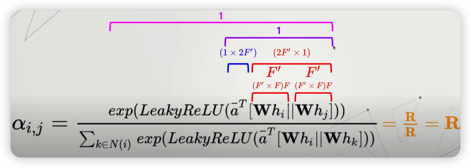
• step 2) SELF-attention

  • \(a: \mathbf{R}^{F^{\prime}} \times \mathbf{R}^{F^{\prime}} \rightarrow \mathbf{R}\).

  • \(e_{i, j}=a\left(\mathbf{W} \cdot \bar{h}_{i}, \mathbf{W} \cdot \bar{h}_{j}\right)\).

    ( \(e_{i,j}\)의 의미 : importance of node j’s features, to node i )

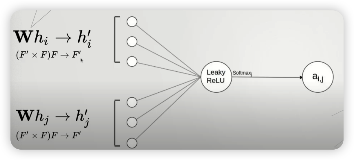
• (상세) Attention mechanism

  • single NN을 사용한다.

  • ex) 만약 node \(i\) 와 node \(j\) 사이의 attention이 이루어진다면….

    

    
    

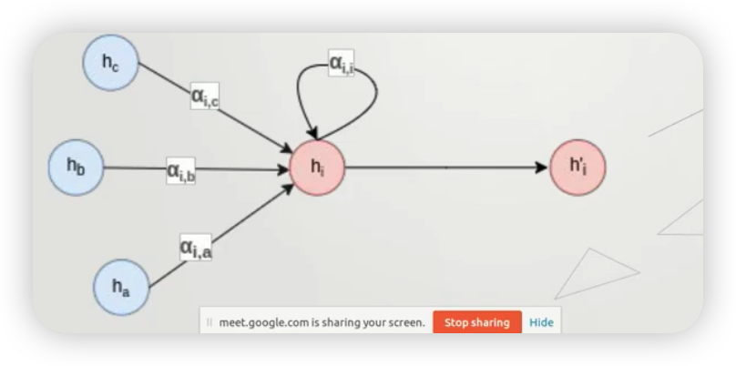
• step 3) update node representaiton

  • 위에서 계산한 attention score를 가중치로 사용하여 이웃 노드들을 조합한다.
  • \(h_{i}^{\prime}=\sigma\left(\sum_{j \in N(i)} \alpha_{i, j} \mathbf{W h} h_{j}\right)\).

  

Multi-head attention

• 위의 step 3)에서, 단지 하나의 head만이 아닌 여러 head를 사용하여, 보다 풍부한 표현을 잡아낼 수 있다.
• Ex) single-head attention
  • \(h_{i}^{\prime}=\sigma\left(\sum_{j \in N(i)} \alpha_{i, j} \mathbf{W h} h_{j}\right)\).
• Ex) multi-head attention - concatenation
  • \(h_{i}^{\prime}= \mid \mid _{k=1}^{K} \sigma\left(\sum_{j \in N(i)} \alpha_{i, j}^{k} \mathbf{W}^{k} h_{j}\right)\).
• Ex) multi-head attention - average
  • \(h_{i}^{\prime}=\sigma\left(\frac{1}{K} \sum_{k=1}^{K} \sum_{j \in N(i)} \alpha_{i, j}^{k} \mathbf{W}^{k} h_{j}\right)\).

GAT의 장점

• (1) computationally efficient
  • 병렬 처리 가능
• (2) different importances 반영 가능
• (3) shared manner to all edges
• (4) transductive & inductive case에 모두 적용 가능

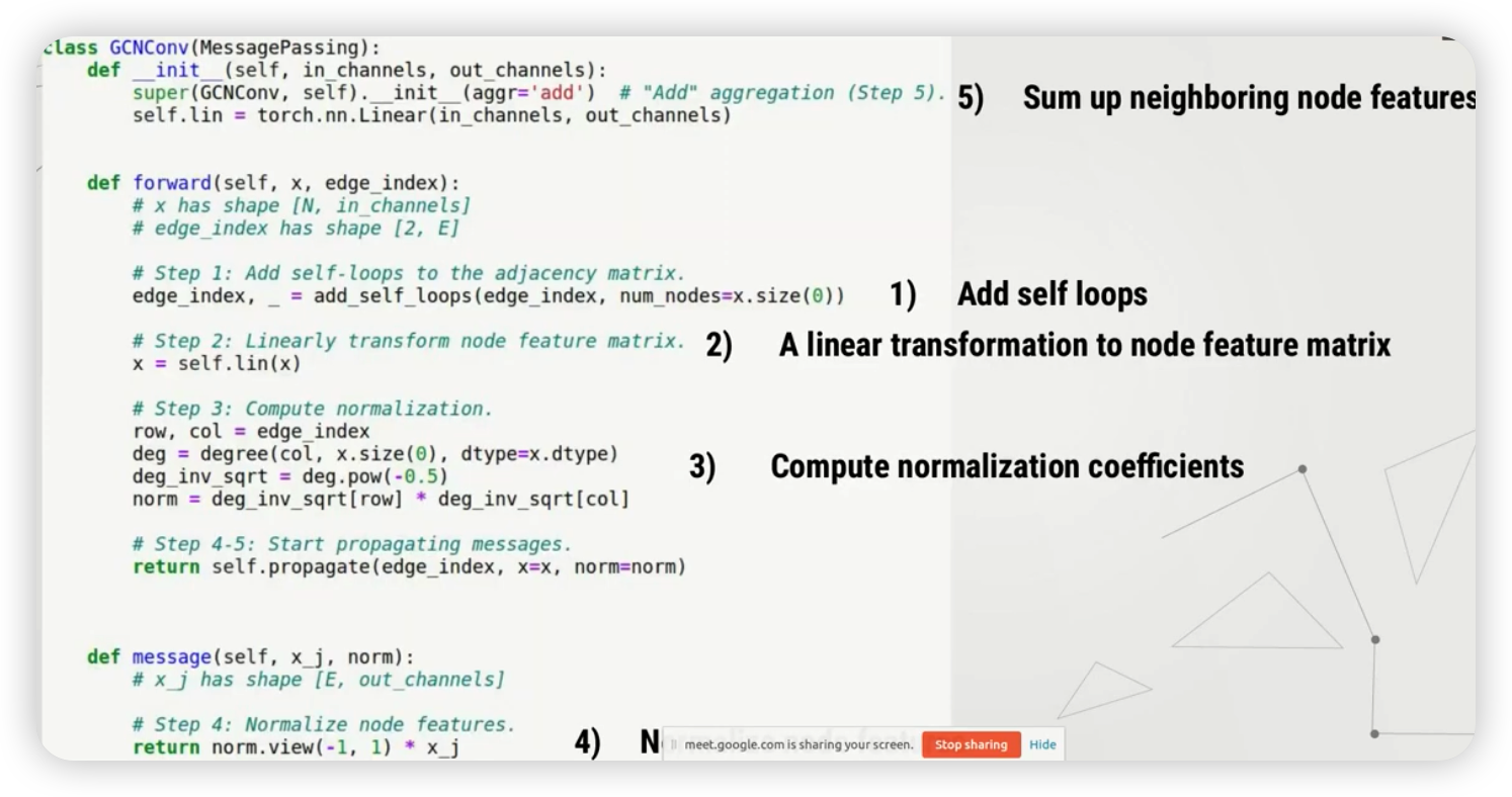
3) 간단한 GCN 구현

\(\mathbf{x}_{i}^{(k)}=\sum_{j \in \mathcal{N}(i) \cup\{i\}} \frac{1}{\sqrt{\operatorname{deg}(i)} \cdot \sqrt{\operatorname{deg}(j)}} \cdot\left(\Theta \cdot \mathbf{x}_{j}^{(k-1)}\right)\).

구현 순서

• (1) add self-loop
• (2) linear transformation ( to node feature matrix )
• (3) compute noramlization coefficients
• (4) normalize node features with 93)
• (5) aggregate (=sum, in GCN) node features

4) Import Packages

import numpy as np
import torch
import torch.nn as nn
import torch.nn.functional as F

5) GAT layer 구현

GAT layer를, torch_geometric의 것을 사용하지말고, 직접 구현해보자

class GATLayer(nn.Module):
    def __init__(self, in_features, out_features, dropout, alpha, concat=True):
        super(GATLayer, self).__init__()
        self.dropout       = dropout        # drop prob = 0.6
        self.in_features   = in_features    # 
        self.out_features  = out_features   # 
        self.alpha         = alpha          # LeakyReLU의 alpha 값
        self.concat        = concat         # concat = True / False

        # Xavier Initialization
        self.W = nn.Parameter(torch.zeros(size=(in_features, out_features)))
        self.a = nn.Parameter(torch.zeros(size=(2*out_features, 1)))
        nn.init.xavier_uniform_(self.W.data, gain=1.414)
        nn.init.xavier_uniform_(self.a.data, gain=1.414)
        
        # Leaky ReLU
        self.leakyrelu = nn.LeakyReLU(self.alpha)

    def forward(self, x, adj):
        #-----------------------------#
        # x : node feature ( num nodes , node_feature_dim )
        # adg : adjacency matrix ( nodes , nodes )
        #-----------------------------#
        # (1) Linear Transformation
        h = torch.mm(input, self.W)
        N = h.size()[0]

        # (2) Attention Mechanism
        a_input = torch.cat([h.repeat(1, N).view(N * N, -1), h.repeat(N, 1)], dim=1).view(N, -1, 2 * self.out_features)
        e       = self.leakyrelu(torch.matmul(a_input, self.a).squeeze(2))

        # (3) Masked Attention
        zero_vec  = -9e15*torch.ones_like(e)
        attention = torch.where(adj > 0, e, zero_vec)
        attention = F.softmax(attention, dim=1)
        attention = F.dropout(attention, self.dropout, training=self.training)
        h_prime   = torch.matmul(attention, h)

        if self.concat:
            return F.elu(h_prime)
        else:
            return h_prime

6) GAT 구현

필요한 Packages 불러오기

• 이번엔, 직접 만든 GAT layer가 아닌, torch_geometric에 내장된 GATConv를 이용할 것이다.

from torch_geometric.data import Data
from torch_geometric.nn import GATConv
from torch_geometric.datasets import Planetoid
import torch_geometric.transforms as T

import matplotlib.pyplot as plt

name_data = 'Cora'
dataset = Planetoid(root= '/tmp/' + name_data, name = name_data)
dataset.transform = T.NormalizeFeatures()

print(f"Number of Classes in {name_data}:", dataset.num_classes)
print(f"Number of Node Features in {name_data}:", dataset.num_node_features)

( 사용하는 dataset은, Chapter 1과 동일한 Cora dataset이다 )

• class 종류 수 : 7
• node feature 차원 : 1433

GAT Layer를 사용한 모델 구현

GATConv의 argument

• arg[0] : input 차원
• arg[1] : output 차원
• arg[2] (heads) : head의 개수
• arg[3] (dropout) : dropout ratio

class GAT(torch.nn.Module):
    def __init__(self):
        super(GAT, self).__init__()
        self.hid = 8
        self.in_head = 8
        self.out_head = 1
        
        # 2개의 GAT layer를 쌓을 것이다.
        # ( 2번째 : multi-head attention 사용 )
        self.conv1 = GATConv(dataset.num_features, self.hid, heads=self.in_head, dropout=0.6)
        self.conv2 = GATConv(self.hid*self.in_head, dataset.num_classes, concat=False,
                             heads=self.out_head, dropout=0.6)

    def forward(self, data):
        x, edge_index = data.x, data.edge_index
        #-------------------------------------#
        # x : (2708, 1433)
        # edge_index : (2, 10556)
        #-------------------------------------#
        x = F.dropout(x, p=0.6, training=self.training)
        x = self.conv1(x, edge_index)
        #-------------------------------------#
        # x : (2708, 64)
        # 64 : hid 차원(8) x head 개수 (8)
        #-------------------------------------#
        x = F.elu(x)
        x = F.dropout(x, p=0.6, training=self.training)
        x = self.conv2(x, edge_index)
        #-------------------------------------#
        # x : (2708, 7)
        #-------------------------------------#
        return F.log_softmax(x, dim=1)

모델 & 옵티마이저 생성

device = torch.device('cuda' if torch.cuda.is_available() else 'cpu')

model = GAT().to(device)
data = dataset[0].to(device)
optimizer = torch.optim.Adam(model.parameters(), lr=0.005, weight_decay=5e-4)  

7) 모델 학습

model.train()
for epoch in range(1000):
    model.train()
    optimizer.zero_grad()
    out = model(data)
    loss = F.nll_loss(out[data.train_mask], data.y[data.train_mask])
    
    if epoch%200 == 0:
        print(loss)
    
    loss.backward()
    optimizer.step()

8) 모델 평가

model.eval()
_, pred = model(data).max(dim=1)
correct = float(pred[data.test_mask].eq(data.y[data.test_mask]).sum().item())
acc = correct / data.test_mask.sum().item()
print('Accuracy: {:.4f}'.format(acc))