(paper) Gated Graph Sequence NN

Gated Graph Sequence NN (2015, 2251)

Contents

1. Abstract
2. Introduction
3. GNN
   1. Propagation Model
   2. Output Model & Learning
4. GGNN (Gated GNN)
   1. Node Annotations
   2. Propagation Model
   3. Output Models
5. GGSNN (Gated Graph Sequence NN)

Abstract

GNN : feature learning technique for graph-structured inputs

this paper : GNN + GRU

1. Introduction

Main Contribution : extension of GNN that outputs SEQUENCES

2 settings for feature learning on graphs

• (1) learning represetnation of INPUT GRAPH
• (2) learning representaiton of INTERNAL SATE during the process of *producing a sequence of outputs8

propose GGS-NNS ( Gated Graph Sequence Neural Networks )

2. GNN

Notation

• graph : \(\mathcal{G}=(\mathcal{V}, \mathcal{E})\)
• node vector : \(\mathbf{h}_{v} \in \mathbb{R}^{D}\)
• node labels : \(l_{v} \in\left\{1, \ldots, L_{\mathcal{V}}\right\}\)
• edge labels : \(l_{e} \in\left\{1, \ldots, L_{\mathcal{E}}\right\}\)

Function

• \(\operatorname{In}(v)=\left\{v^{\prime} \mid\left(v^{\prime}, v\right) \in \mathcal{E}\right\}\) :
  • returns the set of predecessor nodes \(v^{\prime}\) with \(v^{\prime} \rightarrow v\)
• \(\operatorname{OuT}(v)=\left\{v^{\prime} \mid\left(v, v^{\prime}\right) \in \mathcal{E}\right\}\) :
  • returns the set of successor nodes \(v\) with \(v^{\prime} \rightarrow v\)

GNN maps “graphs” to “outputs”, via 2 steps

[1] Propagation step

• computes node representations for each node

[2] Output model

• output model = \(o_{v}=g\left(\mathbf{h}_{v}, l_{v}\right)\)
• maps from node representations and corresponding labels to an output \(o_{v}\)

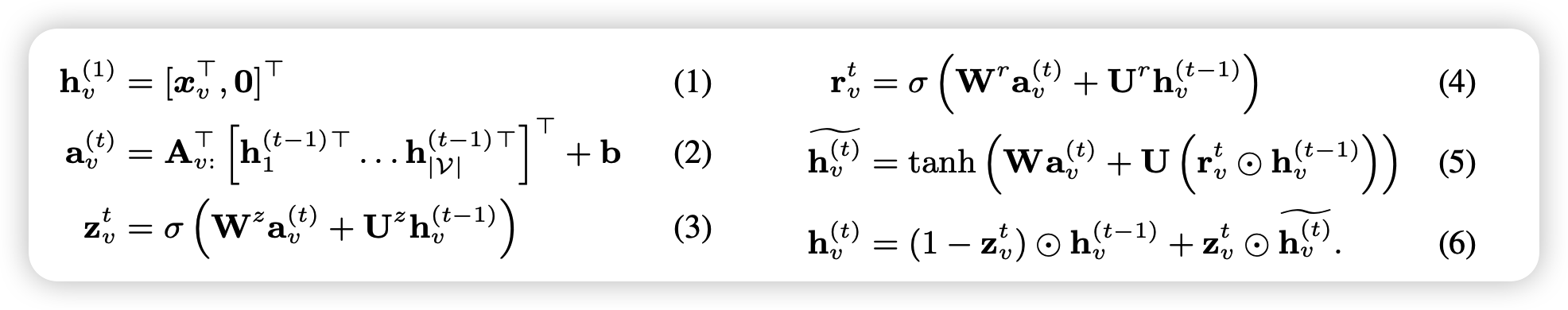
(1) Propagation Model

• iterative procedure
• initial node representation \(\mathbf{h}_{v}^{(1)}\) : arbitrary values
• recurrence :
  • \(\mathbf{h}_{v}^{(t)}=f^{*}\left(l_{v}, l_{\operatorname{CO}(v)}, l_{\operatorname{NBR}(v)}, \mathbf{h}_{\operatorname{NBR}(v)}^{(t-1)}\right)\).

(2) Output Model & Learning

• pass

3. GGNN (Gated GNN)

GNN + GRU

• unroll the recurrence for a fixed number of steps \(T\)

(1) Node Annotations

Unlike GNN…

• incorporate nodel labels as additional inputs

  ( = call them “node annotation” ( \(\boldsymbol{x}\) ) )

How is node annotation used?

• ex) predict wheter node \(t\) can be reached from node \(s\)

(2) Propagation Model

Notation

( \(D\) : dimension of node vector )

( \(\mid \mathcal{V} \mid\) : number of nodes )

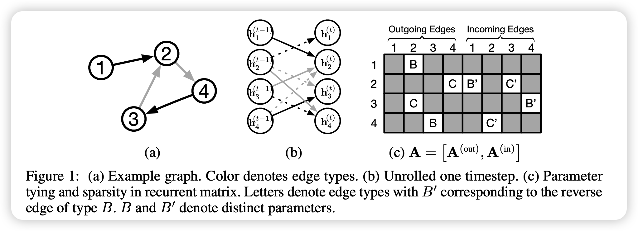
• \(\mathbf{A} \in \mathbb{R}^{D \mid \mathcal{V} \mid \times 2 D \mid \mathcal{V} \mid }\) :
  • determines how nodes in the graph communicate with each other
• \(\mathbf{A}_{v:} \in \mathbb{R}^{D \mid V \mid \times 2 D}\) :
  • two columns of blocks in \(\mathbf{A}^{(\text {out })}\) and \(\mathbf{A}^{(\mathrm{in})}\) corresponding to node \(v\)
• \(\mathbf{a}_{v}^{(t)} \in \mathbb{R}^{2 D}\) :
  • contains activations from edges in both directions

(3) Output Models

( can be several types of one-step outputs )

1. node selection tasks

   • \(o_{v}=g\left(\mathbf{h}_{v}^{(T)}, \boldsymbol{x}_{v}\right)\) for each node \(v\)
   • apply softmax over node scores

2. graph level representation vector :

   • \(\mathbf{h}_{\mathcal{G}}=\tanh \left(\sum_{v \in \mathcal{V}} \sigma\left(i\left(\mathbf{h}_{v}^{(T)}, \boldsymbol{x}_{v}\right)\right) \odot \tanh \left(j\left(\mathbf{h}_{v}^{(T)}, \boldsymbol{x}_{v}\right)\right)\right)\).

     • \(\sigma\left(i\left(\mathbf{h}_{v}^{(T)}, \boldsymbol{x}_{v}\right)\right)\) : soft attention,

       ( that decides which nodes are relevant to the current graph-level task )

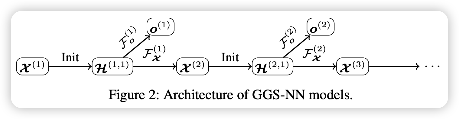
4. GGSNN (Gated Graph Sequence NN)

several GG-NNs operate in sequence, to produce an output sequence \(\boldsymbol{o}^{(1)} \ldots \boldsymbol{o}^{(K)}\)

( for \(k^{th}\) output step )

• matrix of node annotations : \(\mathcal{X}^{(k)}=\left[\boldsymbol{x}_{1}^{(k)} ; \ldots ; \boldsymbol{x}_{ \mid \mathcal{V} \mid }^{(k)}\right]^{\top} \in \mathbb{R}^{ \mid \mathcal{V} \mid \times L_{\mathcal{V}}}\)

use 2 GG-NNs : \(\mathcal{F}_{\boldsymbol{o}}^{(k)}\) & \(\mathcal{F}_{\mathcal{X}}^{(k)}\)

• \(\mathcal{F}_{\boldsymbol{o}}^{(k)}\) : for predicting \(\boldsymbol{o}^{(k)}\) from \(\mathcal{X}^{(k)}\)
• \(\mathcal{F}_{\mathcal{X}}^{(k)}\) : for predicting \(\mathcal{X}^{(k+1)}\) from \(\mathcal{X}^{(k)}\)

( both contain (1) propagation model & (2) output model )

Propagation model

• \(\mathcal{H}^{(k, t)}=\) \(\left[\mathbf{h}_{1}^{(k, t)} ; \ldots ; \mathbf{h}_{ \mid \mathcal{V} \mid }^{(k, t)}\right]^{\top} \in \mathbb{R}^{ \mid \mathcal{V} \mid \times D}\)

  • matrix of node vectors at the \(t^{t h}\) propagation step of the \(k^{t h}\) output step

• \(\mathcal{F}_{\boldsymbol{o}}^{(k)}\) & \(\mathcal{F}_{\mathcal{X}}^{(k)}\) can have single propagation model, and a separate output models

  ( much faster to train & evaluate than full model )

Output model ( Node Annotation output model )

Goal : predict \(\mathcal{X}^{(k+1)}\) from \(\mathcal{H}^{(k, T)}\)

• prediction is done for each node independently,
• using neural network \(j\left(\mathbf{h}_{v}^{(k, T)}, \boldsymbol{x}_{v}^{(k)}\right)\)

Final output : \(\boldsymbol{x}_{v}^{(k+1)}=\sigma\left(j\left(\mathbf{h}_{v}^{(k, T)}, \boldsymbol{x}_{v}^{(k)}\right)\right) .\)

2 training settings

1. specifying all intermediate annotations \(\mathcal{X}^{(k)}\)

   ( = Sequence outputs with observed annotations )

2. training the full model end-to-end, given only \(\mathcal{X}^{(1)}\), graphs and target sequences

   ( = Sequence outputs with latent annotations

   • when intermediate node annotations \(\mathcal{X}^{(k)}\) are not available,

     treat them as hidden units in the network )