
[ 12. Frequent Subgraph Mining with GNNs ]
( 참고 : CS224W: Machine Learning with Graphs )
Contents
-
12-1. Subgraphs & Motifs
- 12-2. Neural Subgraph Matching
- 12-3. Mining Frequent Subgraphs
1. Subgraphs & Motifs
(1) Introduction
def ) “building blocks” of networks
- can “characterize” & “discriminate” networks
example :
(2) Subgraphs
2 ways to formalize subgraphs
- 1) “NODE”-induced subgraph
- 2) “EDGE”-induced subgraph
a) “NODE”-induced subgraph
- subset of the NODES & all edges induced by the nodes
- called “induced subgraph”
- example )
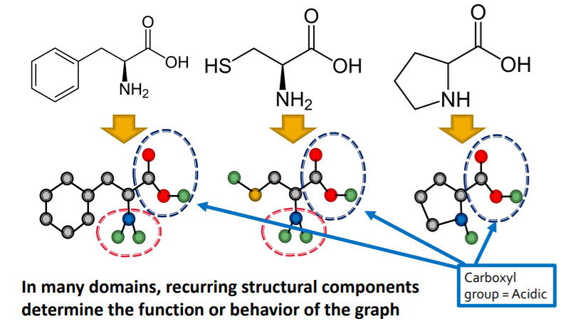
- Chemistry ( functional groups )
- \[V^{\prime} \subseteq V\]
- \[E^{\prime}=\left\{(u, v) \in E \mid u, v \in V^{\prime}\right\}\]
- \[G^{\prime} \text { is the subgraph of } G \text { induced by } V^{\prime}\]
b) “EDGE”-induced subgraph
- subset of the EDGES & all corresponding nodes
- called “non-induced subgraph” / “subgraph”
- example )
- Knowledge graphs (focus on edges representing logical relations)
\(G^{\prime}=\left(V^{\prime}, E^{\prime}\right) \text { is an edge induced subgraph iff }\).
- \(E^{\prime} \subseteq E\).
- \(V^{\prime}=\left\{v \in V \mid(v, u) \in E^{\prime} \text { for some } u\right\}\).
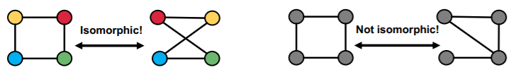
c) Graph Isomorphism
check whether 2 graphs are identical!
[ Definition ]
-
\(G_{1}=\left(V_{1}, E_{1}\right)\) and \(G_{2}=\left(V_{2}, E_{2}\right)\) are isomorphic …
if there exists a bijection \(f: V_{1} \rightarrow V_{2}\) such that \((u, v) \in\) \(E_{1}\) iff \((f(a), f(b)) \in E_{2}\)
( + \(f\) is called the isomorphism )
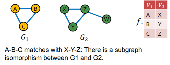
d) Subgraph Isomorphism
[ Definition ]
-
\(G_2\) is subgraph isomorphic to \(G_1\) ….
if some “subgraph of \(G_2\)” is isomorhic to \(G_1\)
( = \(G_1\) is a subgraph of \(G_2\) )
\(\rightarrow\) NP-hard problem
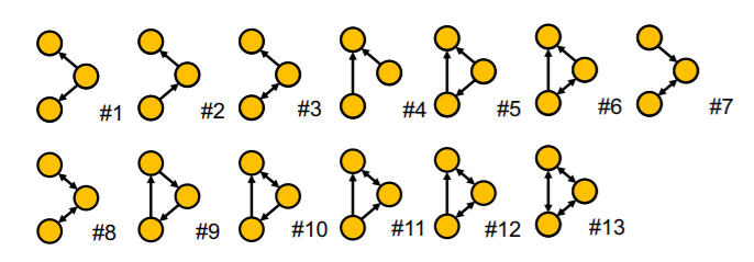
e) Examples
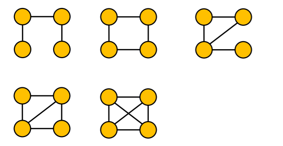
non-isomorphic + connected + undirected + size 4
non-isomorphic + connected + directed + size 3
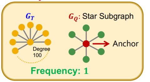
(3) Network Motifs
“(1) recurring, (2) significant (3) patterns of interconnections”
Definition
-
(1) Recurring : # of frequency
\(\rightarrow\) “how to define frequency?”
-
(2) Significant : more frequent than random graph
\(\rightarrow\) “how to define random graph?”
-
(3) Pattern : small (node-induced) subgraph
Why do we need motifs?
- Help us understand how graphs work
- Help us make predictions based on presence or lack of presence in a graph dataset
a) Subgraph FREQUENCY (SF)
Notation
- \(G_T\) : Target graph ( = big graph )
- \(G_Q\) : Query graph ( = small graph )
[ Graph-level SF ]
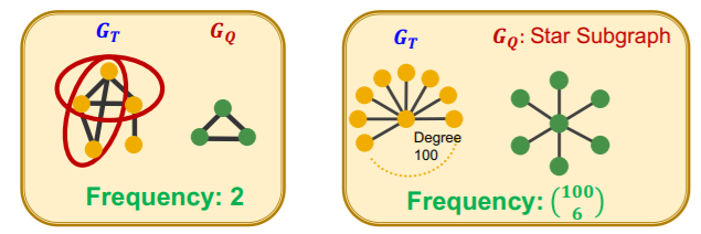
[ Node-level SF ]
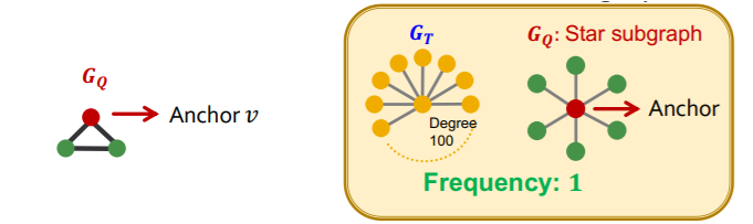
- \((G_Q,v)\) : “node-anchored” subgraph
- robust to outliers
Want to find out “frequency of multiple subgraphs” in dataset!
\(\rightarrow\) treat \(G_T\) as a large dataset, with “disconnected components” ( = individual graphs )
b) Motif SIGNIFICANCE
more frequent than null-model ( = random model )
\(\rightarrow\) so, how to define “RANDOM graphs”?
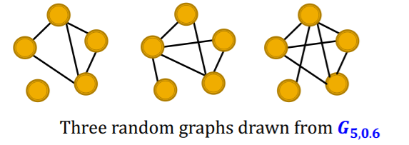
[ Erdos-Renyi (ER) random graphs ]
- \(G_{n,p}\) : undirected graph / \(n\) nodes / edge probability of \(p\)
-
can be disconnected
-
example :
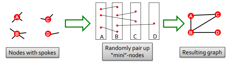
[ Configuration Model ]
-
goal : generate random graph…
- with \(N\) nodes
- with degree \(k_1, \cdots k_N\)
-
compare
- (1) \(G^{\text{real}}\)
- (2) \(G^{\text{random}}\)
( both have same degree sequence! )
Overview
-
intuition : Motifs are overrepresented in a network when compared to random graphs
-
3 step
-
step 1) count motifs in \(G^{\text{real}}\)
-
step 2) generate random graph
-
with similar statistics
( ex. nodes / edges / degree sequences)
-
-
step 3) use statistical measures to evaluate “significance of each motif”
- ex) Z-score
-
Z-score :
- \(Z_i\) : captures “significance” of motif \(i\)
- \(Z_{i}=\left(N_{i}^{\mathrm{real}}-\bar{N}_{i}^{\mathrm{rand}}\right) / \operatorname{std}\left(N_{i}^{\mathrm{rand}}\right)\).
- \(N_{i}^{\text {real }}\) : # (motif \(i\) ) in graph \(G^{\text {real }}\)
- \(\bar{N}_{i}^{\text {rand }}\) : average #(motifs \(i\) ) in random graph
- Network significance profile (SP) : normalized Score
Network significance profile (SP) :
- \(S P_{i}=Z_{i} / \sqrt{\sum_{j} Z_{j}^{2}}\).
- vector of “normalized Z-scores”
- dimension = # of types of motifs
- meaning : relative significance of subgraphs
2. Neural Subgraph Matching
(1) Subgraph Matching
Question : is QUERY graph a subgraph of TARGET graph?
- QUERY graph : connected
- TARGET graph : can be disconnected
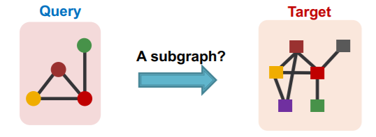
use GNN to “predict” subgraph isomorphism
-
binary prediction
-
use embeddings to decide if neighborhood of \(u\) is isomorphic to subgraph of neighborhood of \(v\)
-
do not only predict its existence,
but also identify corresponding nodes \(u\) & \(v\)
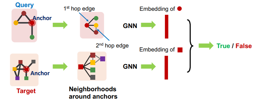
a) Decomposing graphs ( into neighborhoods )
- 1) for each node in \(G_T\) ….
- obtain a k-hop neighborhood around the anchor
- 2) for each node in \(G_Q\) ….
- same
- 3) embed all those neighborhoods with GNN
- By computing the embeddings for the anchor
b) Order Embedding Space
- mapping : graph \(A\) \(\rightarrow\) point \(Z_A\)
- \(Z_A\) is non-negative in all dimensions
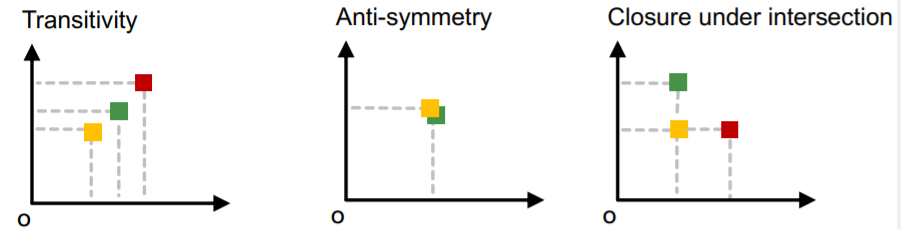
- key point : Transitivity
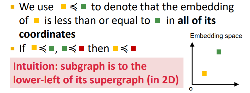
- Example
Why “order embedding space”?
-
1) transitivity
-
if \(G_1\) is a subgraph of \(G_2\) and \(G_2\) is a subgraph of \(G_3\)
\(\rightarrow\) then \(G_1\) is a subgraph of \(G_3\)
-
-
2) anti-symmetry
-
if \(G_1\) is a subgraph of \(G_2\) and \(G_2\) is a subgraph of \(G_1\)
\(\rightarrow\) then \(G_1\) is isomorphic to \(G_2\)
-
-
3) closure under intersection
c) Order constraint
- What loss function should we use, so that the learned order embedding reflects the subgraph relationship?
- design loss functions based on the order constraint
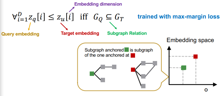
d) Max-margin Loss
-
optimize by minimizing “Max-margin loss”
-
margin between \(G_q\) & \(G_t\)
= \(E\left(G_{q}, G_{t}\right)=\sum_{i=1}^{D}\left(\max \left(0, z_{q}[i]-z_{t}[i]\right)\right)^{2}\)
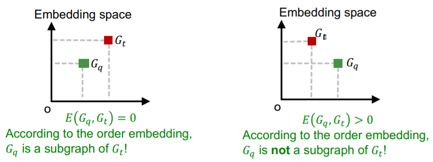
\(E\left(G_{q}, G_{t}\right)=0\), when \(G_{q}\) is a subgraph of \(G_{t}\)
\(E\left(G_{q}, G_{t}\right)>0\), when \(G_{q}\) is not a subgraph of \(G_{t}\)
Trained in a way that…
- 1) positive examples :
- minimize \(E(G_q, G_t)\), when \(G_q\) is a subgraph of \(G_t\)
- 2) negative examples :
- minimize \(\text{max}(0,\alpha-E(G_q,G_t))\)
3. Mining Frequent Subgraphs
(1) Representation Learning
Goal : find most frequent size-\(k\) motifs!
Process
- 1) enumerate all size-\(k\) connected subgraphs
- 2) count # of each subgraph types
But computationally hard….
\(\rightarrow\) use “REPRESENTATION learning”
how?
-
task 1) Combinatorial explosion
solution 1) organize the search space
-
task 2) Subgraph isomorphism
solution 2) prediction using GNN
Settings
- \(G_T\) : target graph
- \(k\) : size parameter
- \(r\) : desired number of results ( = TOP \(r\) graphs )
Task
-
among all possible graphs of \(k\) nodes,
identify top \(r\) graphs with highest frequency in \(G_T\)
-
use “node-level” definition
(2) SPMiner
a) overview
-
SPMiner = neural model to identify frequent motifs
-
procedure
- step 1) decompose
- decompose into subgraphs
- overlapping node-anchored neighborhoods ( ex. 2-hop )
- step 2) encoder
- embed subgraphs
- caution : to “order embedding” space
- can quickly find out the frequency of a given subgraph \(G_Q\)
- step 3) search procedure
- find frequent subgraphs, by “growing patterns”
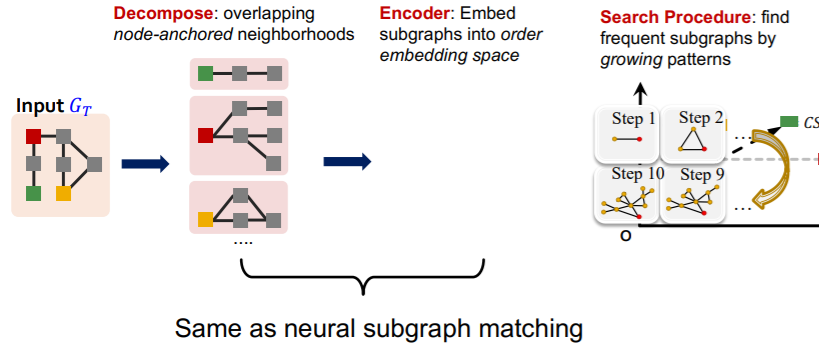
- step 1) decompose
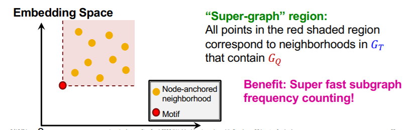
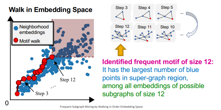
b) Motif Frequency Estimation with SPMiner
\(G_{N_i}\) = set of subgraphs of \(G_T\)
Task :
- estimate frequency of \(G_Q\) ( = query graph = motif = red dot )
- by counting the number of \(G_{N_i}\) ( = yellow dot )
- such that their embeddings \(Z_{N_i}\) satisfy \(Z_Q \leq Z_{N_i}\)
[ Search Procedure ]
- step 1) randomly select starting node \(u\) in \(G_T\)
- set \(S=\{u\}\)
- step 2) Grow a motif iteratively…
- choose a neighbor of node in \(S\) & add it to \(S\)
- grow motifs to find larger motifs
- step 3) Terminate
- when reached a desired motif size
- tesult : “subgraph of target graph induced by \(S\)”
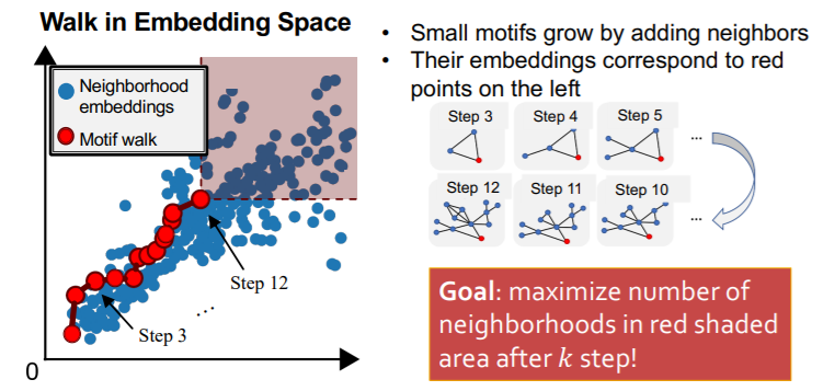
[ Choosing the next node ]
-
Total Violation of a subgraph \(G\)
= # of neighborhoods, that do not contain \(G\)
= # of neighborhoods, that do not satisfy \(Z_Q \leq Z_{N_i}\)
-
minimizing Total Violation
= maximizing frequency
-
use “GREEDY strategy”
- at every step, add node that gives “smallest total violation”