(CS224W) 13.Community Detection in Networks

[ 13. Community Detection in Networks ]

( 참고 : CS224W: Machine Learning with Graphs )

Contents

• 13-1. Community Detection in Networks
• 13-2. Network Communities
• 13-3. Louvain Algorithm
• 13-4. Detecting Overlapping Communities : BigCLAM

1. Community Detection in Networks

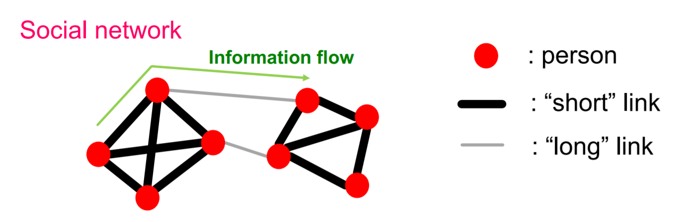
(1) Flow of Information

• people are “embedded” in social network
• Information flows through links
  • 1) short link
  • 2) long link

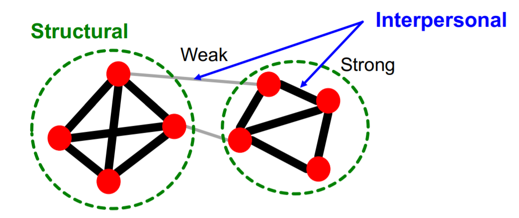
(2) Two perspective of friendships

1) Structural

• span different parts of the network
• ex) group (A), group (B), ..

2) Interpersonal

• friendship between person (a) & person (b)
• ex) strong, weak

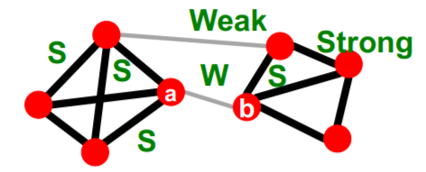
(3) Granovetter’s Explanation

connection between the (1) social and (2) structural role of an edge

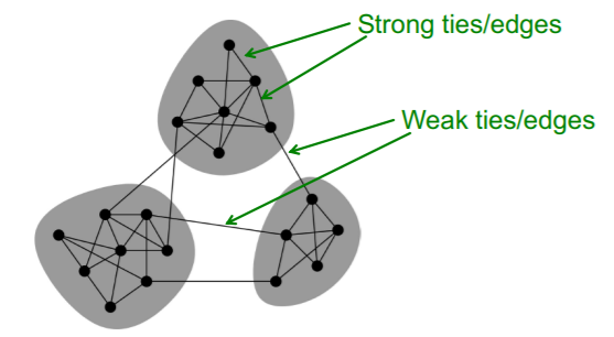
1) Structure

• Structurally embedded (tightly-connected) edges = socially STRONG
• Long-range edges = socially WEAK

2) Information

• Structurally embedded (tightly-connected) edges = heavily REDUNDANT
• Long-range edges = allows to gather new INFORMATION

(4) Triadic Closure

key idea : if (A&B) and (B&C) \(\rightarrow\) (A&C) is likely!

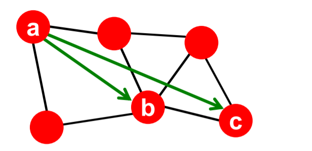
Triadic closure = High clustering coefficient

[ Intuition ]

if B and C both have “friend A” in common…

• 1) B is more likely to meet C
• 2) B & C trust each other
• 3) A has incentive to bring B & C together

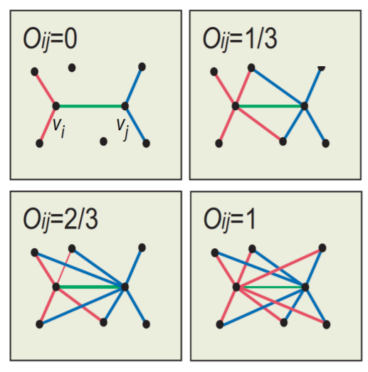
(5) Edge Overlap

\(O_{i j}=\frac{ \mid (N(i) \cap N(j))-\{i, j\} \mid }{ \mid (N(i) \cup N(j))-\{i, j\} \mid }\).

• \(N(i)\) : neighbors of node \(i\)

(6) Conceptual Picture of Networks

2. Network Communities

(1) Granovetter’s theory

Networks = composed of “tightly connected set of nodes”

Network Communities

• lots of internal connections
• few external connections

\(\rightarrow\) so, how to “automatically find densely connected groups”?

(2) Social Network Data

Examples

• Zachary’s Karate Club network
• Micro-Markets in Sponsored Search
• NCAA Football network

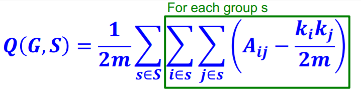
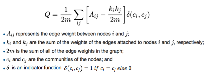
(3) Modularity \(Q\)

Modularity = measure of “how well a network is PARTITIONED” into communities

• small communities ( disjoint networks ) : \(s \in S\)

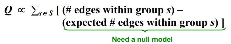
Null model = “Configuration Model”

• settings :
  • graph : \(G\)
  • # of nodes : \(n\)
  • # of edges : \(m\)
• construct rewired network \(G^{'}\)

Expected number of edges between nodes \(i\) & \(j\) ( of degrees \(k_i\) & \(k_j\) )

= \(k_{i} \cdot \frac{k_{j}}{2 m}=\frac{k_{i} k_{j}}{2 m}\).

• \(2m\) : # of directed edges

Expected number of edges in (multigraph) \(G^{'}\) :

\(\begin{aligned} &=\frac{1}{2} \sum_{i \in N} \sum_{j \in N} \frac{k_{i} k_{j}}{2 m}=\frac{1}{2} \cdot \frac{1}{2 m} \sum_{i \in N} k_{i}\left(\sum_{j \in N} k_{j}\right)= \\ &=\frac{1}{4 m} 2 m \cdot 2 m=m \end{aligned}\).

Modularity of partitioning \(S\) of graph \(G\)

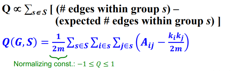
• range : [ -1 ~ 1 ]
• if positive, number of edges within group exceeds the expected number

• greater than 0.3~0.7 : significant community structure

• both applicable to “weighted & unweighted” networks

Reformulation :

3. Louvain Algorithm

(1) Introduction

• “Greedy” algorithm
• work both for “weighted & unweighted” graphs
• provides “Hierarchical” communities
• details
  • fast
  • rapid convergance
  • high modularity output

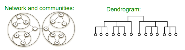
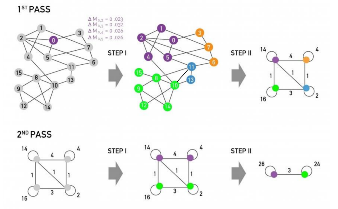
(2) 2 Phases

[ Phase 1 ] Modularity is optimized by allowing only local changes to node-communities memberships

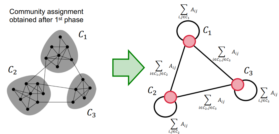
[ Phase 2 ] The identified communities are aggregated into super-nodes to build a new network

Phase 1

• step 1) set each node as “distinct community”
• step 2) for ( \(i\) in ALL_NODES ) :
  • compute \(\Delta Q\) , when putting node \(i\) into “community of neighbor \(j\)”
  • change the community of \(i\) to node \(j\), which gives the largest gain in \(\Delta Q\)
• run until no movement

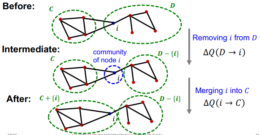
Modularity Gain, \(\Delta Q\)

settings : “move node \(i\) from community \(D\) to \(C\) “

• \(\Delta Q(D \rightarrow i \rightarrow C)=\Delta Q(D \rightarrow i)+\Delta Q(i \rightarrow C)\).

How to calculate \(\Delta Q(i \rightarrow C)\) ?

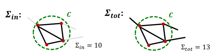
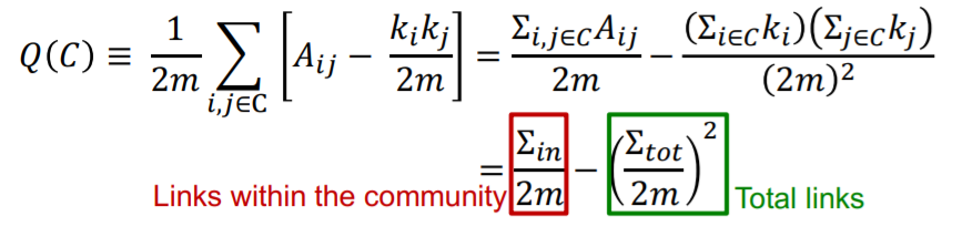
• step 1) calculate \(Q(C)\) ( = modularity within \(C\) )

  • Notation
    • \(\boldsymbol{\Sigma}_{\boldsymbol{i n}} \equiv \sum_{i, j \in C} A_{i j}\) : ~ link “BETWEEN” nodes in \(C\)
    • \(\boldsymbol{\Sigma}_{\boldsymbol{t o t}} \equiv \sum_{i \in C} k_{i}\) : ~ link “ALL” nodes in \(C\)

  

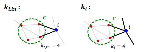
• step 2) calculate \(k_{i,in}\) & \(k_{i}\)

  • Notation

    • \(\boldsymbol{k}_{\boldsymbol{i}, \boldsymbol{i n}} \equiv \sum_{j \in C} A_{i j}+\sum_{j \in C} A_{j i}\) : sum of link BETWEEN node \(i\) & \(C\)
    • \(\boldsymbol{k}_i\) : sum of ALL link of node \(i\)

    

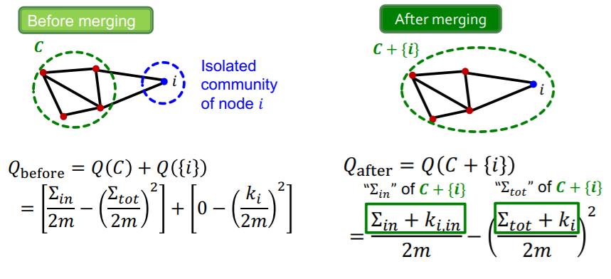
• step 3) calculate \(Q_{before}\) & \(Q_{after}\)

• step 4) calculate \(\Delta Q(i \rightarrow C)\)

  \(\Delta Q(i \rightarrow C)= Q_{\text {after }}-Q_{\text {before }} \\ =\left[\frac{\Sigma_{i n}+k_{i, i n}}{2 m}-\left(\frac{\Sigma_{t o t}+k_{i}}{2 m}\right)^{2}\right] -\left[\frac{\Sigma_{i n}}{2 m}-\left(\frac{\Sigma_{t o t}}{2 m}\right)^{2}-\left(\frac{k_{i}}{2 m}\right)^{2}\right]\).

  ( calculate \(\Delta Q(D \rightarrow i)\) in the same way )

(3) Summary

[ Phase 1 ]

• calculate \(C^{\prime}=\operatorname{argmax}_{\mathrm{C}}, \Delta Q\left(C \rightarrow i \rightarrow C^{\prime}\right)\)
• if \(\Delta Q\left(C \rightarrow i \rightarrow C^{\prime}\right)>0\), then update
  • \(C \leftarrow C-\{i\}\).
  • \(C^{\prime} \leftarrow C^{\prime}+\{i\}\).

[ Phase 2 ]

• communities obtained in the first phase are contracted into super-nodes
• then, do the same as [ Phase 1 ] on the super-node network

4. Detecting Overlapping Communities : BigCLAM

(1) Overlapping Communities

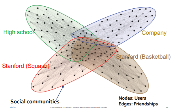
(2) Plan of Action

step 1) Community Affiliation Graph Model (AGM)

• define a “GENERATIVE” model for graphs
• based on “node community affiliations”

step 2) for a given graph \(G\)…

• assume \(G\) was generated by AGM
• find the best AGM

(3) Community AGM

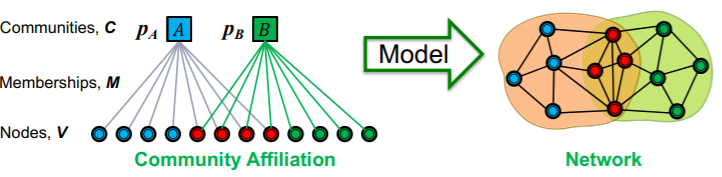
Model parameters

• node \(V\), community \(C\), membership \(M\)
• each community has a single probability \(p_c\)

Can express a variety of community structures

• ex) non-overlapping, overlapping, nested

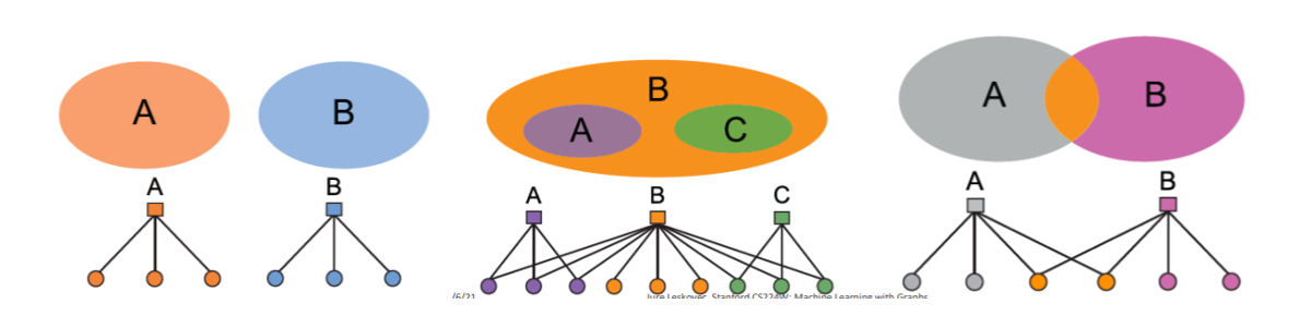
generative process

• \(p_c\) : nodes in community \(c\), connect to each other by probability \(p_c\)
• \(p(u, v)=1-\prod_{c \in M_{u} \cap M_{v}}\left(1-p_{c}\right)\),
  • since multiple communities!

(4) Detecting Communities

how to detect communities with AGM?

\(\rightarrow\) given a GRAPH, find a MODEL \(F\)

• optimize using MLE

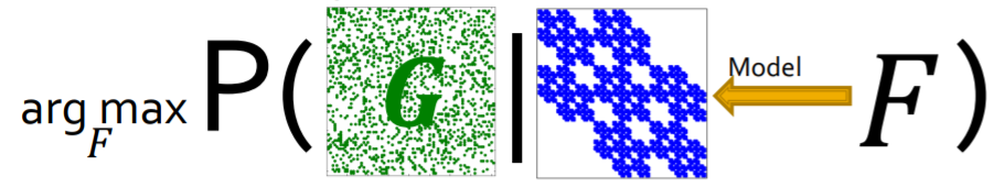
• efficiently calculate \(P(G\mid F)\)

Graph Likelihood , \(P(G\mid F)\)

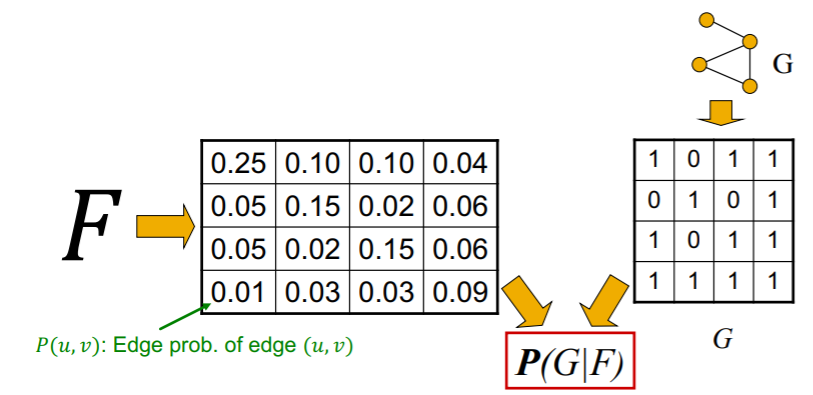
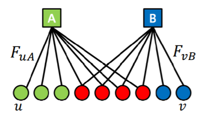
Strengths of membership

\(F_{uA}\) : membership strength, of node \(u\) to community \(A\)

• \(F_{uA}=0\) : NO membership

\(P_C(u,v)\) : probability \(u\) &\(v\) are connected (for community \(C\))

• \(P_{C}(u, v)=1-\exp \left(-F_{u C} \cdot F_{v C}\right)\).
  • \(F_{uC}\) & \(F_{vC}\) : non-negative
• valid probability : [ 0 ~ 1 ]

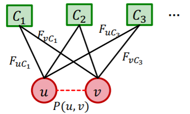
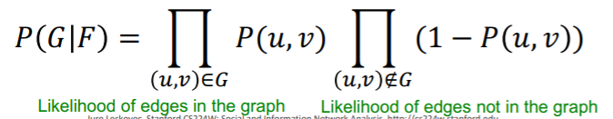
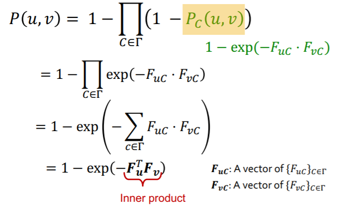
\(P(u,v)\) : probability \(u\) &\(v\) are connected (for at least one communities)

• \(P(u, v)=1-\prod_{C \in \Gamma}\left(1-P_{C}(u, v)\right)\).

• expand..

  

(5) BigCLAM

Key idea :

• Probability of nodes \(u\) & \(v\) linking

  = proportional to the strength of shared memberships

  ( \(\mathbf{P}(\boldsymbol{u}, \boldsymbol{v})=\mathbf{1}-\boldsymbol{\text { exp }}\left(-\boldsymbol{F}_{\boldsymbol{u}}^{\boldsymbol{T}} \boldsymbol{F}_{v}\right)\) )

• given \(G(V, E)\), maximize likelihood of \(G\) , under \(F\)

Likelihood

\(\begin{aligned} P(G \mid F) &=\prod_{(u, v) \in E} P(u, v) \prod_{(u, v) \notin E}(1-P(u, v)) \\ &=\prod_{(u, v) \in E}\left(1-\exp \left(-F_{u}^{T} F_{v}\right)\right) \prod_{(u, v) \notin E} \exp \left(-F_{u}^{T} F_{v}\right) \end{aligned}\).

Log Likelihood

\(\begin{aligned} &\log (P(G \mid \boldsymbol{F})) \\ &=\log \left(\prod_{(u, v) \in E}\left(1-\exp \left(-\boldsymbol{F}_{u}^{T} \boldsymbol{F}_{v}\right)\right) \prod_{(u, v) \notin E} \exp \left(-\boldsymbol{F}_{u}^{T} \boldsymbol{F}_{v}\right)\right) \\ &=\sum_{(u, v) \in E} \log \left(1-\exp \left(-\boldsymbol{F}_{u}^{T} \boldsymbol{F}_{v}\right)\right)-\sum_{(u, v) \notin E} \boldsymbol{F}_{u}^{T} \boldsymbol{F}_{v} \\ &\equiv \ell(\boldsymbol{F}): \text { Our objective } \end{aligned}\).

Optimization

• goal : optimize \(\ell(\boldsymbol{F})\)

• start with random \(F\)

• iterate until convergence

  • “gradient ascent”
  • partial derivative :
    • \(\nabla \ell(\boldsymbol{F})=\sum_{v \in \mathcal{N}(u)}\left(\frac{\exp \left(-\boldsymbol{F}_{u}^{T} \boldsymbol{F}_{v}\right)}{1-\exp \left(-\boldsymbol{F}_{u}^{T} \boldsymbol{F}_{v}\right)}\right) \cdot \boldsymbol{F}_{v}-\sum_{v \notin \mathcal{N}(u)} \boldsymbol{F}_{v}\).

• solution for Time Complexity :

  

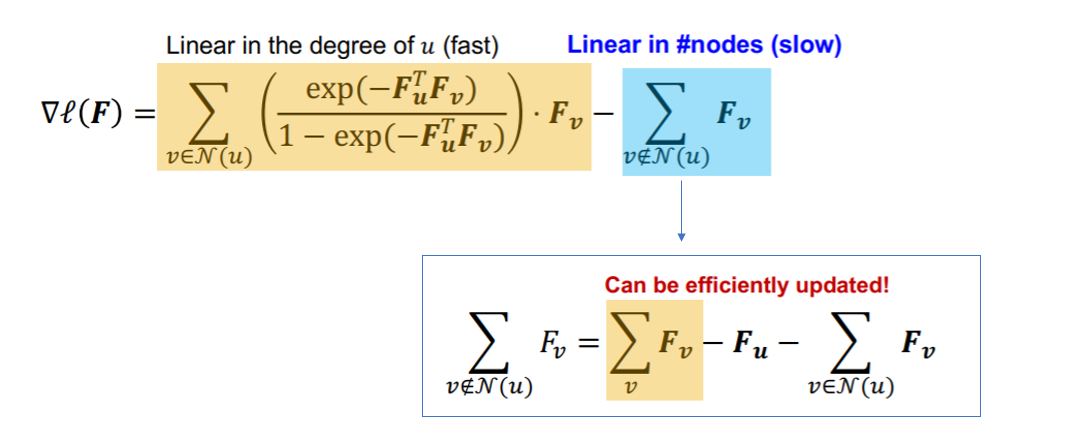
  • \(\sum_{v} \boldsymbol{F}_{v}\) : can be computed at the beginning!