(CS224W) 14.Traditional Generative Models for Graphs

[ 14. Traditional Generative Models for Graphs ]

( 참고 : CS224W: Machine Learning with Graphs )

Contents

1. Properties of Real-world Graphs
2. Erdos-Renyi Random Graphs
3. The Small-world Model
4. Kronecker Graph Model
5. Summary

Graph Generative models

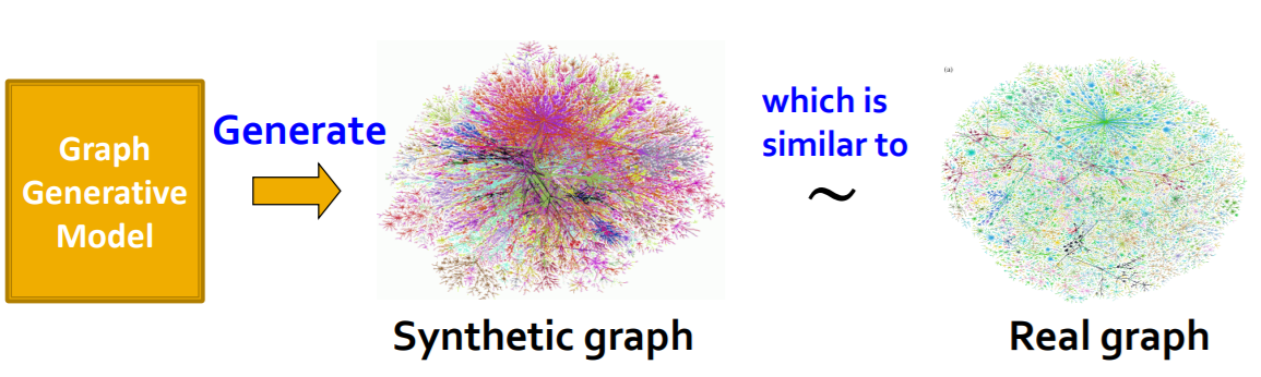
Why is it needed?

1. Insights : understand ‘formulation of graph’
2. Predictions : predict how the ‘graph will evolve’
3. Simulations
4. Anomaly detection

Road map of Graph Generation

[1] Properties of Real-world Graphs

• properties for successful graph generative model

[2] Traditional graph generative models

• assumption on graph formulation process
• ex) Erdos-Renyi Random Graphs

[3] Deep graph generative models

• (in lecture 15)

1. Properties of Real-world Graphs

(1) Key Network properties

1. Degree distribution : \(P(k)\)
2. Clustering coefficient : \(C\)
3. Connected components : \(s\)
4. Path length : \(h\)

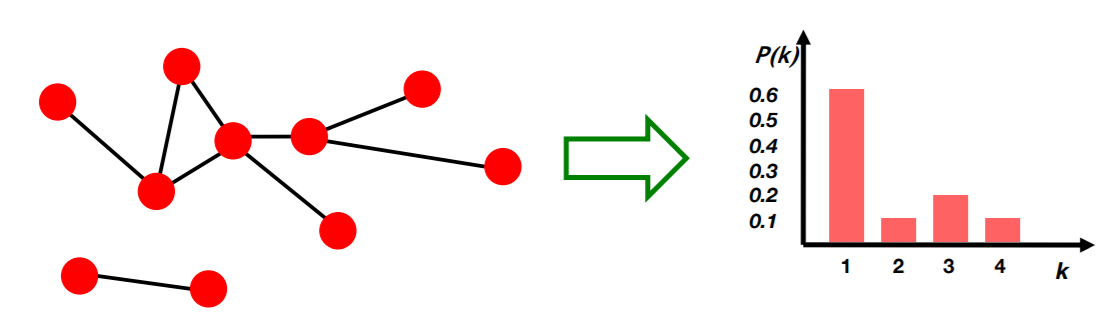
a) Degree distribution : \(P(k)\)

probability that a randomly chosen node has degree k

• Notation :
  • \(N_k\) : # of nodes with “degree k”
  • \(P(k)\) : normalized version ( = \(N_k / N\) )

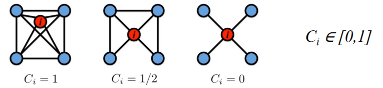
b) Clustering coefficient : \(C\)

how are node \(i\)’s’ neighbors connected to each other?

• Notation

  • \(k_i\) : degree of node \(i\)
  • \(C_i\) : clustering coefficient of node \(i\) ( = \(\frac{2e_i}{k_i(k_i-1)}\) )
    • \(e_i\) = # of edges between the “node \(i\)’s’ neighbors”

• Example :

  

Graph Clustering Coefficient?

• take average of all “node clustering coefficient” ( \(C = \frac{1}{N}\sum_{i=1}^{N}C_i\) )

c) Connected components : \(s\)

Size of the “LARGEST connected component”

• Connected component : set where any two nodes can be joined by a path
• How to find “connected component”?
  • step 1) select random node
  • step 2) BFS (Breadth-First Search)
    • label all the visited nodes
    • visited nodes are connected
  • step 3) if unvisited nodes exists,
    • repeat step 1) & step 2)

d) Path length : \(h\)

Diameter = maximum (shortest path) distance between “ANY” pair of nodes

• Notation
  • \(h_{ij}\) : distance from node \(i\) & \(j\)
  • \(E_{max}\) : max # of possible edges ( = \(n(n-1)/2\) )
  • \(\bar{h}\) : Average path length
• Average path length :
  • \(\bar{h}=\frac{1}{2 E_{\max }} \sum_{i, j \neq i} h_{i j}\).

(2) Case Study : MSN graph

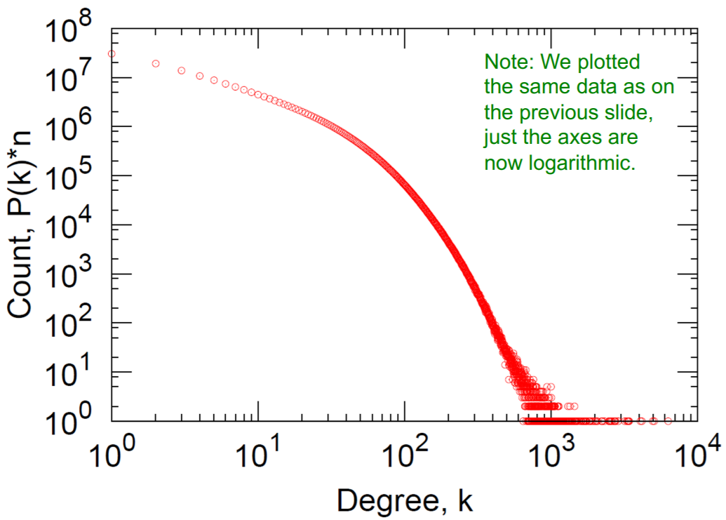
a) Degree distribution

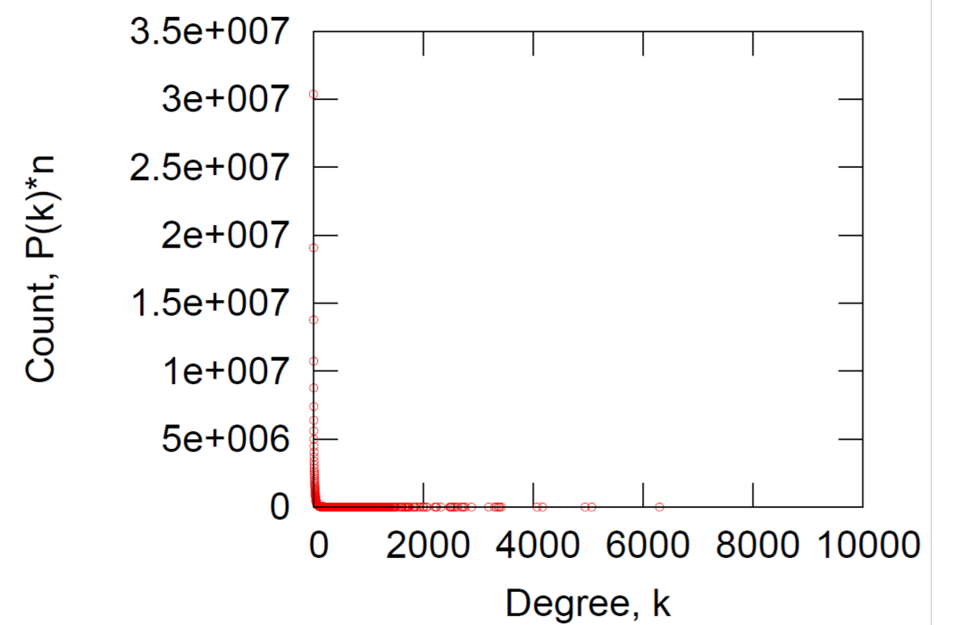
Log-Log Degree distribution

b) Clustering coefficient

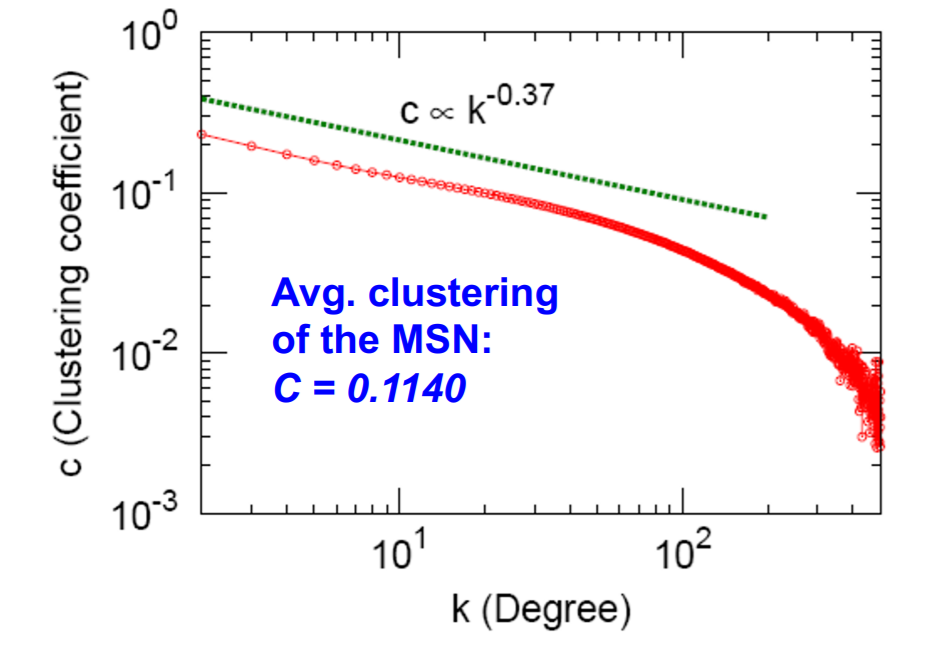
\(C_k\) : “average \(C_i\), of nodes \(i\) with degree k”

• \(C_k = \frac{1}{N}\sum_{i:k_i=k}^{}C_i\).

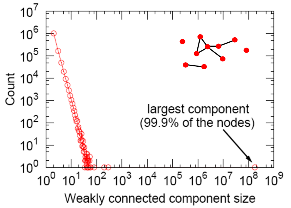
c) Connected Components

d) Path Length

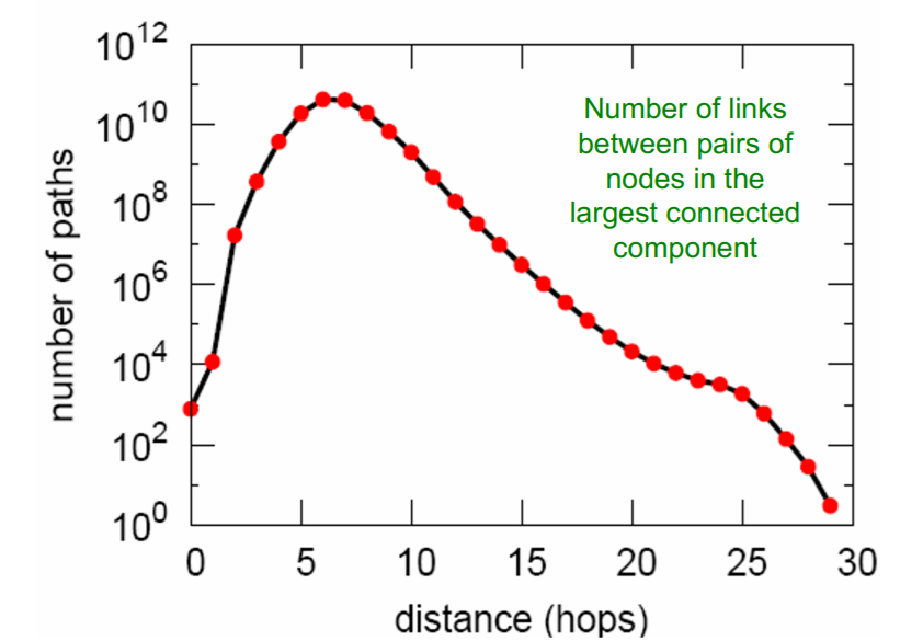
• Average Path Length = 6.6

• 90% of nodes can be reached in \(< 8\) hops

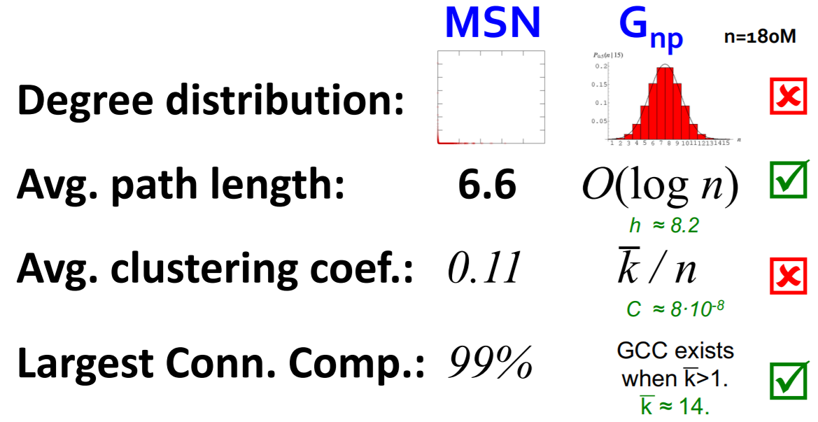
Summary

• a) Degree distribution : heavily skewed (avg degree=14.4)
• b) Clustering coefficient : 0.11
• c) Connectivity : giant component (99%)
• d) Path length : 6.6

Question : so, is it a surprising/expected result?

\(\rightarrow\) need a NULL model

2. Erdos-Renyi Random Graphs

(1) Introduction

• Simplest model of graphs

• Two variants

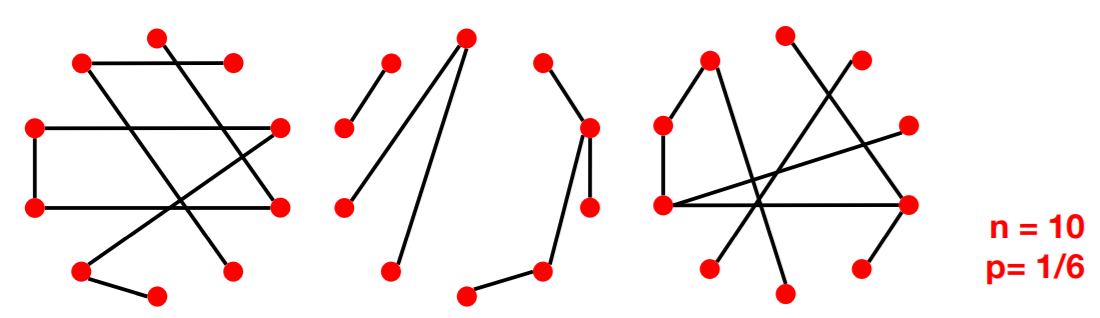
  • 1) \(G_{np}\) : \(n\) nodes & prob \(p\) of connected
  • 2) \(G_{nm}\) : \(n\) nodes & \(m\) edges

  \(\rightarrow\) expected edges are same, but 1) is stochastic, 2) is deterministic

  ( = 1) is “RANDOM” graph model / not unique )

(2) Random Graph model \(G_{np}\)

Properties of \(G_{np}\)

• 1) Degree distribution : \(P(k)\)
• 2) Clustering coefficient : \(C\)
• 3) Connected Component : \(s\)
• 4) Path length : \(h\)

(3) Degree distribution : \(P(k)\)

Binomial Distribution : \(k \sim \text{Binom}(n-1,p)\)

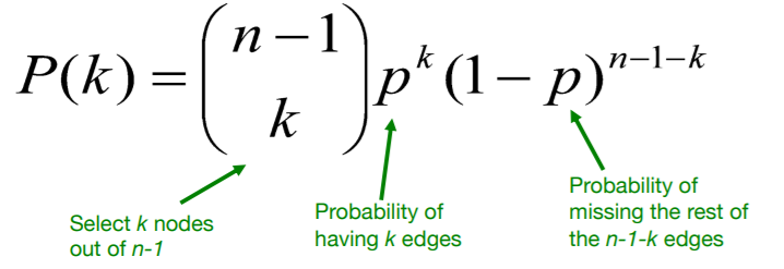
• mean : \(\bar{k}=p(n-1)\).
• variance : \(\sigma^{2}=p(1-p)(n-1)\)

(4) Clustering coefficient : \(C\)

Clustering coefficient : \(C_{i}=\frac{2 e_{i}}{k_{i}\left(k_{i}-1\right)}\)

• \(k_i\) : degree of node \(i\)

Expected \(\boldsymbol{e}_i\) : \(\mathrm{E}\left[\boldsymbol{e}_{\boldsymbol{i}}\right] =p \frac{k_{i}\left(k_{i}-1\right)}{2}\)

• 1) \(p\) : prob of connection
• 2) \(\frac{k_{i}\left(k_{i}-1\right)}{2}\) : # of distinct pairs of neighbors of node \(i\) of degree \(k_i\)

\[E\left[C_{i}\right]=\frac{p \cdot k_{i}\left(k_{i}-1\right)}{k_{i}\left(k_{i}-1\right)}=p=\frac{\bar{k}}{n-1} \approx \frac{\bar{k}}{n}\]

• 1) clustering coefficient of random graph is SMALL
• 2) fixed average degree + bigger graph \(\rightarrow\) decrease of \(C\)

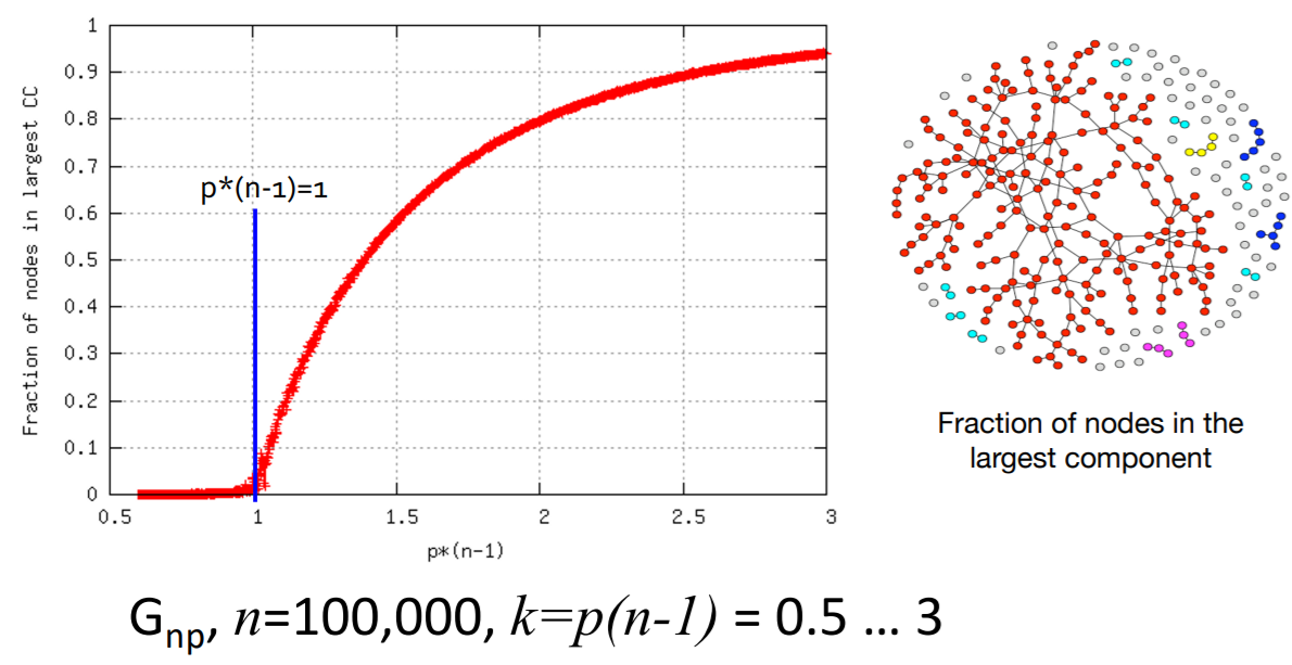
(5) Connected Component of \(G_{np}\)

How does “change of \(p\)” influence the “graph structure”?

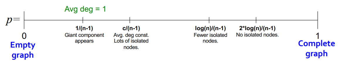
Giant component occurs ( = GCC exists ) , when…

\(\rightarrow\) average degree \(k\) is bigger than 1

(6) Path length : \(h\)

need to know the notion of “EXPANSION”

Expansion

• graph \(G(V,E)\) has expansion \(\alpha\) =

  if \(\forall S \subseteq V\), # of edges leaving \(S \geq \alpha \cdot \min (\mid S \mid, \mid V \backslash S \mid)\)

• that is…

  \[\alpha=\min _{S \subseteq V} \frac{\text { #edges leaving } S}{\min ( \mid S \mid , \mid V \backslash S \mid )}\]

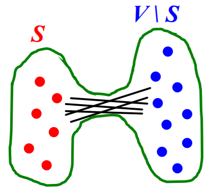
Meaning :

• measure of “robustness”
• to disconnect \(l\) nodes, we need to cut \(\geq \alpha \cdot l\) edges

Example :

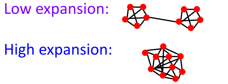
Details

• graph with \(n\) nodes & \(\alpha\) expansion

  = for all pairs of nodes, “there is a path of length \(O((log n)/\alpha)\)“

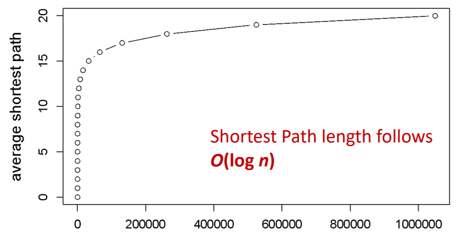
Shortest path of \(G_{np}\)

• ER random graph can grow very large, but nodes will be just a few hops apart

(7) MSN vs \(G_{np}\)

3. The Small-world Model

(1) Motivation for small-world

Trade-off of “clustering coefficient” & “diameter”?

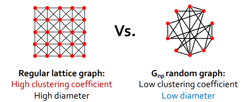
\(\rightarrow\) can we have “HIGH clustering” & “LOW(SHORT) diameter” ?

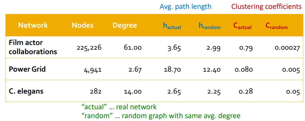
Real networks have “HIGH clustering”

• ex) MSN have \(7\) times higher \(C\) than \(G_{np}\)

Examples :

(2) Interpolate “regular lattice” & “\(G_{np}\)”

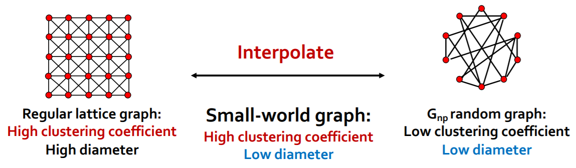
Solution : “Small-world Model”

[Step 1] start with low-dim regular lattice

• high clustering coefficient

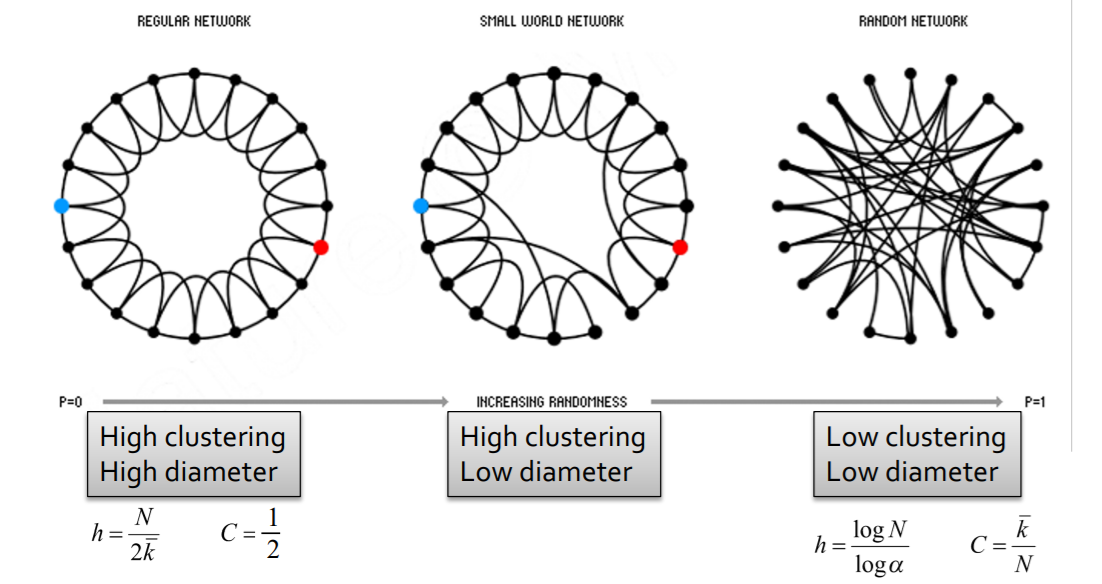
[Step 2] REWIRE

• introduce randomness (shortcuts)

  • add/remove edges ( to join remote parts )

    ( with prob \(p\) )

• enables “interpolation between 2 types of graphs”

4. Kronecker Graph Model

Think of network structure recursively! ( key : self-similarity )

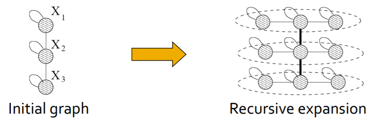
\(\rightarrow\) by using “Kronecker product”

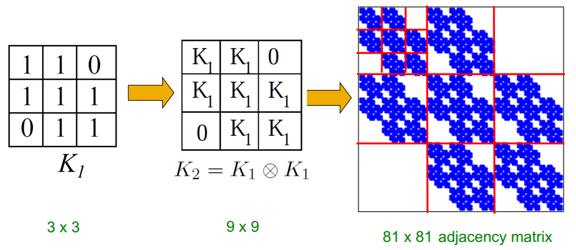
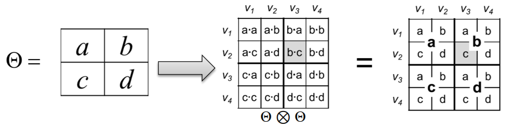
(1) Kronecker Product

\(\mathbf{C}=\mathbf{A} \otimes \mathbf{B} \doteq\left(\begin{array}{cccc} a_{1,1} \mathbf{B} & a_{1,2} \mathbf{B} & \ldots & a_{1, m} \mathbf{B} \\ a_{2,1} \mathbf{B} & a_{2,2} \mathbf{B} & \ldots & a_{2, m} \mathbf{B} \\ \vdots & \vdots & \ddots & \vdots \\ a_{n, 1} \mathbf{B} & a_{n, 2} \mathbf{B} & \ldots & a_{n, m} \mathbf{B} \end{array}\right)\).

• Kronecker product of two graphs

= Kronecker product of their adjacency matrices

• \(K_{1}^{[\mathrm{m}]}=K_{\mathrm{m}}=\underbrace{K_{1} \otimes K_{1} \otimes \ldots K_{1}}_{\mathrm{m} \text { times }}=K_{\mathrm{m}-1} \otimes K_{1}\).

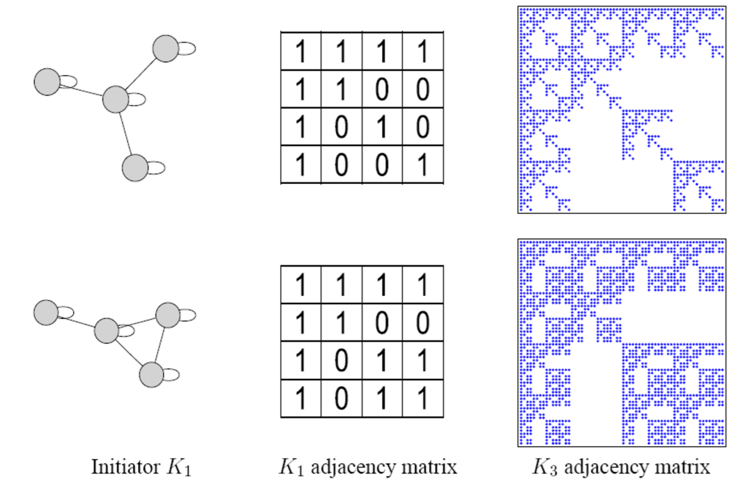
(2) Kronecker Graph

“recursive” model of network structure

(3) Stochastic Kronecker Graph

[Step 1] create \(N_1 \times N_1\) probability matrix \(\Theta_1\)

[Step 2] compute \(k^{th}\) Kronecker power \(\Theta_k\)

[Step 3] include edge \((u,v)\) , with prob \(p_{uv}\)

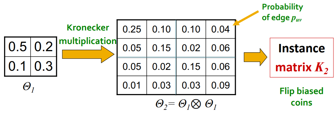
(4) Generation of Kronecker Graphs

Just as “coin flip”!

• exploit the recursive structure of Kronecker graph

5. Summary

Traditional graph generative models

• 1) Erdös-Renyi graphss
• 2) Small-world graphs
• 3) Kronecker graphs

\(\rightarrow\) they all have an assumption ofgraph generation processes