(CS224W) 15.Deep Generative Models for Graphs

[ 15. Deep Generative Models for Graphs ]

( 참고 : CS224W: Machine Learning with Graphs )

Contents

1. ML for Graph Generation
2. GraphRNN : Generating Realistic Graphs
3. BFS (Breadth-First Search node ordering)
4. Evaluating Generated Graphs
5. Application of Deep Graph Generative Models

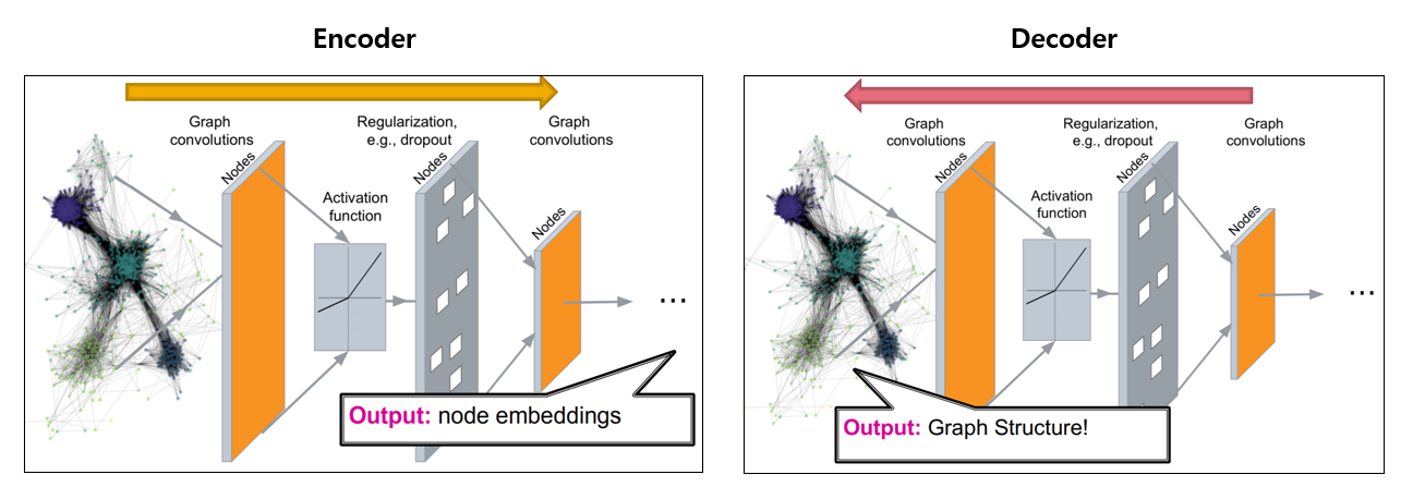
Deep graph encoders & DECODERS

1. ML for Graph Generation

(1) Tasks

[ Task 1 ] Realistic graph generation

• generate graph, that are “similar to a given set of graphs”

[ Task 2 ] Goal-directed graph generation

• for specific objective! ( with constraints )

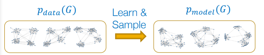
(2) Graph Generative Models

Given : graphs \(\{x_i\}\) ( sampled from \(p_{data}(G)\) )

• we do not have true distribution, but only some samples of it

Goal

• goal 1) learn \(p_{model}(G)\)
• goal 2) sample from \(p_{model}(G)\)

(3) Basics for generative models

Notation

• \(p_{data}(x)\) : data distribution
  • unknown, but have some samples of it ( \(x_i \sim p_{data}(x)\) )
• \(p_{model}(x ; \theta)\) : model
  • use this to approximate \(p_{data}(x)\)

Goal

1. Density estimation
   • make \(p_{model}(x ; \theta)\) close to \(p_{data}(x)\)
2. Sampling
   • \[x_i \sim p_{model}(x ; \theta)\]

a) Density estimation

key point : MLE

• \(\boldsymbol{\theta}^{*}=\underset{\boldsymbol{\theta}}{\arg \max } \mathbb{E}_{x \sim p_{\text {data }}} \log p_{\text {model }}(\boldsymbol{x} \mid \boldsymbol{\theta})\).
• finding a model, that is most likely to have generated the observed \(x\)

b) Sampling

goal : sample from a “complex distribution”

most common approach

• step 1) sample from noise : \(\boldsymbol{z}_{i} \sim N(0,1)\)

• step 2) transform the noise : \(x_{i}=f\left(z_{i} ; \theta\right)\)

  \(\rightarrow\) key point : use \(f(\cdot)\) with DNN

(4) Deep Generative Models

Auto-regressive models

use “chain rule”

• \(p_{\text {model }}(\boldsymbol{x} ; \theta)=\prod_{t=1}^{n} p_{\text {model }}\left(x_{t} \mid x_{1}, \ldots, x_{t-1} ; \theta\right)\).

• (for GNN) \(x_t\) : \(t\)-th action

  • ex) adding NODE, adding EDGE

2. GraphRNN : Generating Realistic Graphs

(1) Basic Idea

generate graphs, by sequentially adding nodes/edges

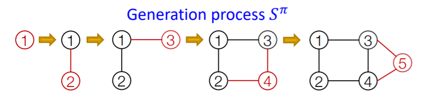
(2) Model graphs as “SEQUENCES”

Notation

• \(G\) : graph
• \(\pi\) : node ordering
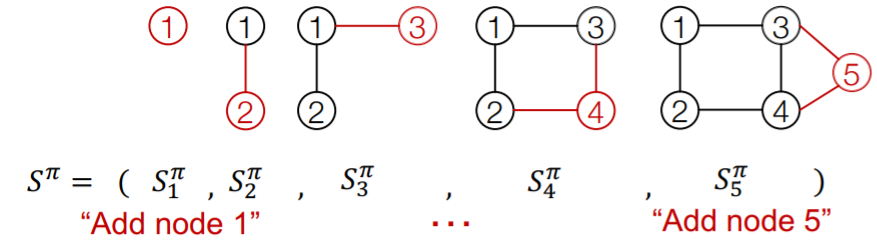
• \(S^{\pi}\) : Sequence

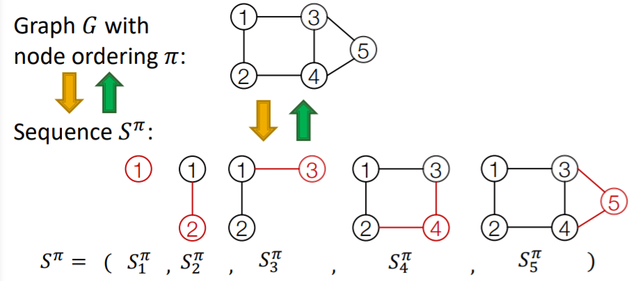
Sequence \(S^{\pi}\) : consists of “2-level”

• 1) node-level : add one node
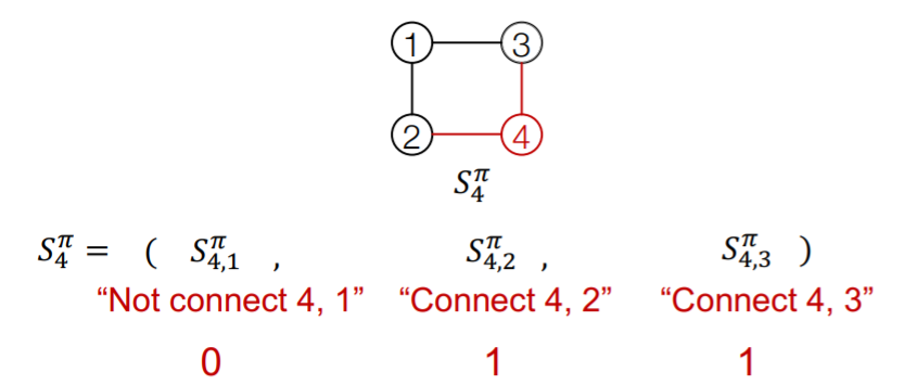
• 2) edge-level : add edge between existing nodes

each “node-level” step is an “edge-level sequence”

• node-level (a)
  • edge-level (a-1)
  • edge-level (a-2)
  • ..
• node-level (b)
  • edge-level (b-1)
  • edge-level (b-2)
  • ..

Ex) node-level

Ex) edge-level

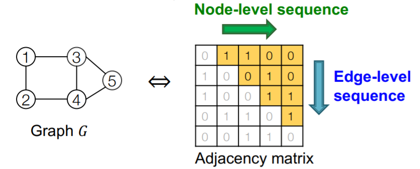
Summary : graph + node ordering = sequence of sequence

• \(\therefore\) graph generation = sequence generation
• ( node ordering : select randomly )

Process : need to model 2 processes

• 1) node-level sequence

  • generate a “state for a new node”

• 2) edge-level sequence

  • generate edges for “new node”, based on its state

  \(\rightarrow\) use RNN for these 2 processes

(3) Graph RNN : 2-level RNN

a) 2-level RNN

1. NODE-level RNN ( nRNN )
2. EDGE-level RNN ( eRNN )

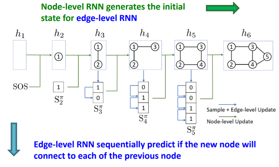
Relation between 2 RNNs :

• “nRNN” generates the initial state for “eRNN”
• “eRNN” sequentially predicts if the new node will connect to each of the previous node

b) key questions

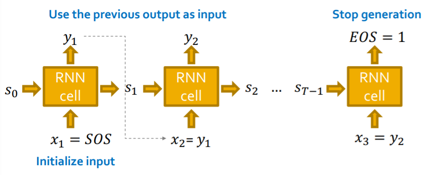
Q1) how does RNN generate sequences?

\(\rightarrow\) let \(x_{t+1} = y_t\) ( input = previous output )

Q2) how to initialize input sequence

\(\rightarrow\) uses SOS token ( zero/one vector )

Q3) when to stop generation?

\(\rightarrow\) use EOS token as extra RNN output

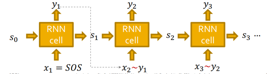
c) deterministic & stochastic

Deterministic output

Stochastic output

Autoregressive Model ( with RNN )

• \(\prod_{k=1}^{n} p_{\operatorname{model}}\left(x_{t} \mid x_{1}, \ldots, x_{t-1} ; \theta\right)\).
• notation : \(y_{t}=p_{\text {model }}\left(x_{t} \mid x_{1}, \ldots, x_{t-1} ; \theta\right)\)
• sampling : \(y_{t}: x_{t+1} \sim y_{t}\)
• how to make it stochastic?
  • output of RNN = “probability of an edge”
  • (1) sample from that distribution & (2) feed to next step

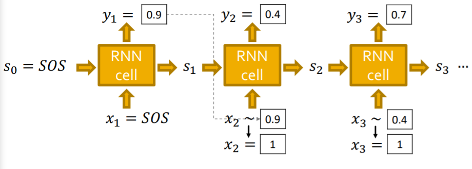
d) RNN at Test Time

Notation

• \(y_t\) : output of RNN at time \(t\)
  • follows “Bernoulli distn”
• \(p\) : probability of an edge
  • (value=1 of prob \(p\)) & (value=0 of prob \(1-p\))

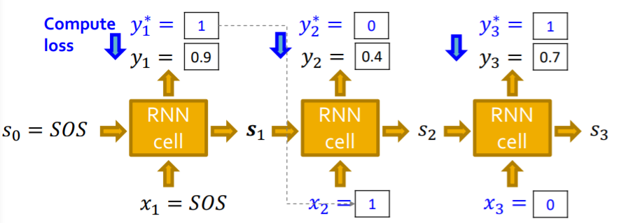
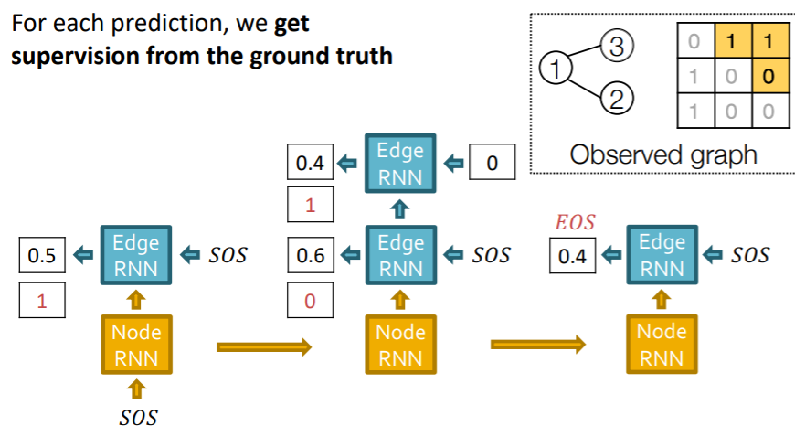
e) RNN at Training Time

observed data (given)

• sequence \(y^{*}\) of edges ( 1 or 0 )

use “Teacher forcing”

• use the “TRUE value”, while training
• loss function : \(L=-\left[y_{1}^{*} \log \left(y_{1}\right)+\left(1-y_{1}^{*}\right) \log \left(1-y_{1}\right)\right]\)

f) Summary

• step 1) add a new node

  • run Node RNN

    ( output of Node RNN = initialize Edge RNN )

• step 2) add new edges ( for new node )

  • run Edge RNN

    ( predict if “new node” connect to “previous node” )

• step 3) add a new node

  • run Node RNN

    ( use last hidden state of Edge RNN )

• step 4) stop generation

  • stop, if Edge RNN outputs EOS at step 1

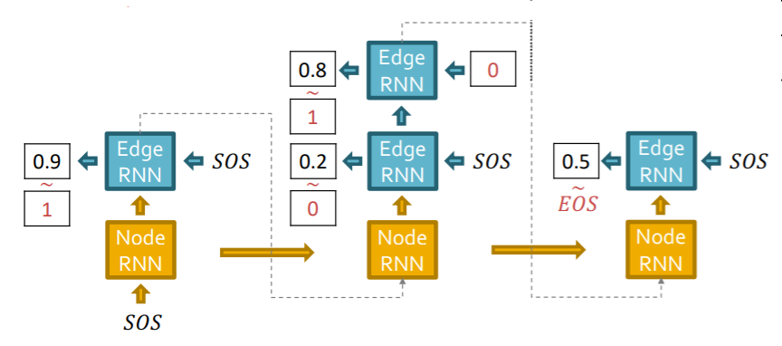
Test time

( just replace “input” at each step, with “GraphRNN’s own predictions” )

3. BFS (Breadth-First Search node ordering)

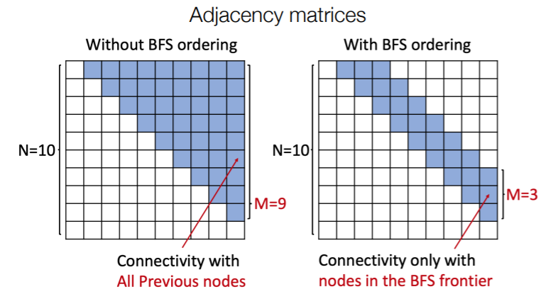
How to get tractability?

too many steps are need for edge generation

• problem 1) need “FULL” adjacency matrix
• problem 2) complex “TOO-LONG” edge dependencies

\(\rightarrow\) Solution : BFS (Breadth-First Search node ordering)

BFS (Breadth-First Search node ordering)

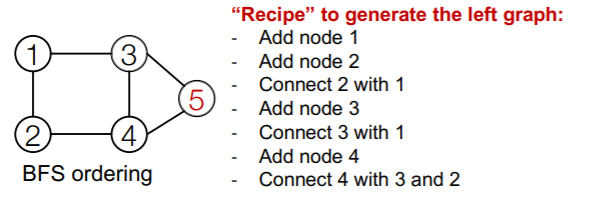
if node \(T\) doesn’t connect to node \(K\) ( \(K<T\) ),

then node \(T+\alpha\) doesn’t ~

( neighbors of \(K\) have already been traversed! )

\(\rightarrow\) only need memory of “2 steps” ( not n-1 steps )

With & Without BFS

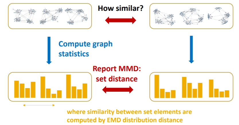
4. Evaluating Generated Graphs

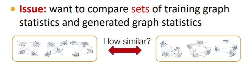
compare 2 sets of graphs

\(\rightarrow\) how much are they similar? need to define “SIMILARITY METRIC”

Solution

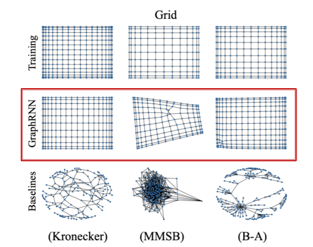
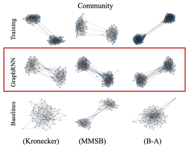
• 1) visual similarity
• 2) graph statistics similarity

(1) Visual similarity

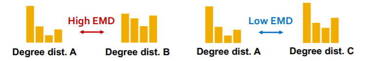
(2) Graph statistics similarity

Typical graph statistics

• 1) degree distribution
• 2) clustering coefficient distribution
• 3) orbit count statistics

\(\rightarrow\) each statistic is “not a scalar”, but “PROBABILITY DISTN”

Solution

• step 1) compare “2 graph statistics”
  • by EMD (Earth Mover Distance)
• step 2) compare “sets of graph statistics”
  • by MMD (Maximum Mean Discrepancy)

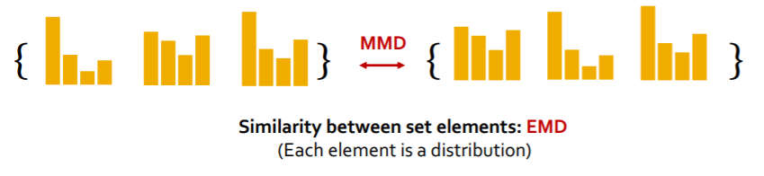
a) EMD

• similarity between “2 distns”
• “minimum effort” that move earth from “one pile to another pile”

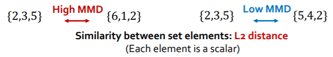
b) MMD

• similarity between “2 sets”,

  based on the similarity between “set elements”

we will compare “2 sets of graph statistics”

( = “2 sets of distributions” )

Summary

• step 1) compute “graph statistics” of all graphs
• step 2) calculate “MMD” ( distance between sets )

5. Application of Deep Graph Generative Models

pass