(CS224W) 16.Advanced Topics in GNNs

[ 16. Advanced Topics in GNNs ]

( 참고 : CS224W: Machine Learning with Graphs )

Contents

1. Review (GNN Training Pipeline)
2. Limitations of GNNs

0. Review (GNN Training Pipeline)

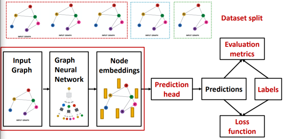
\(\rightarrow\) goal : ‘How can we make GNN representation, MORE EXPRESSIVE?’

1. Limitations of GNNs

(a) perfect GNN

Review

• \(k\)-layer GNN = embeds node, based on “K-hop” neighbors

Perfect GNN

= “injective function” between “neighborhood structure” & “embedding”

• (issue 1) if 2 nodes have SAME neighborhood

  \(\rightarrow\) must have SAME embedding

  

• (issue 2) if 2 nodes have DIFFERENT neighborhood

  \(\rightarrow\) must have DIFFERENT embedding

  

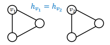
(b) Imperfect existing GNNs

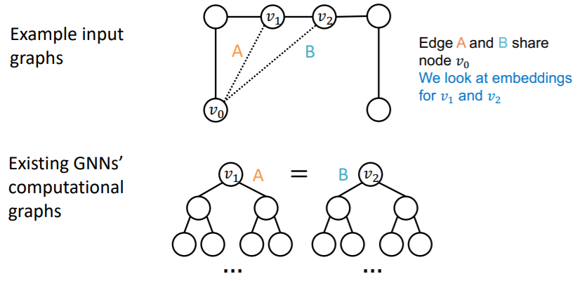
Problem of (issue 1)

• SAME neighborhood, but may want DIFFERENT embeddings!
• ex) road network \(\rightarrow\) called “Position-aware task”

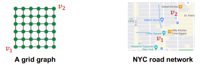
\(\rightarrow\) create node embedding, based on their “POSITIONS” in the graph

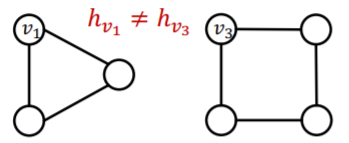
Problem of (issue 2)

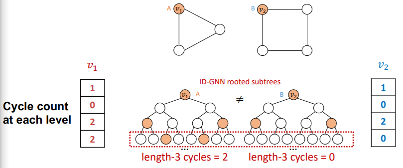
• message passing GNNs cannot count “cycle length”
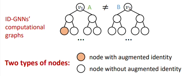
• ex) Identity-aware GNNs

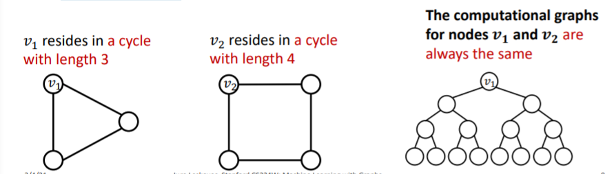
\(\rightarrow\) build message passing GNNs that are more expressive than WL test

Setting

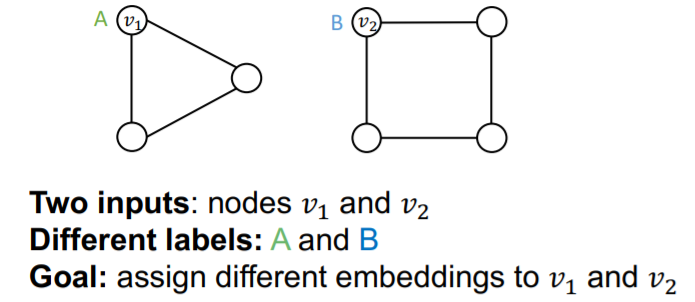
• successful model : DIFFERENT embedding for \(v_1\) & \(v_2\)
• failed model : SAME embedding for \(v_1\) & \(v_2\)

Naive solution : one-hot encoding

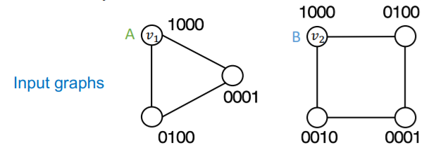
\(\rightarrow\) problem : need \(O(N)\) feature dimension & unable to generalize to new node

2. Position-aware GNN

2 types of tasks

• 1) Structure-aware task : labeled by their “structural roles”
• 2) Position-aware task : labeled by their “position”

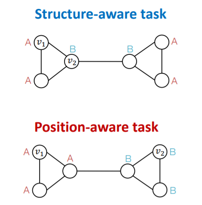
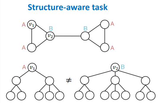
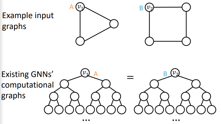
(1) Structure-aware Tasks

• existing GNNs works well!

  ( = able to differentiate \(v_1\) & \(v_2\) )

• how? by using “different computational graphs”

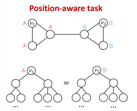
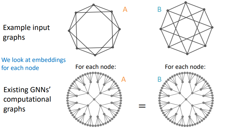
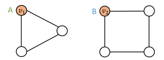
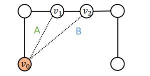
(2) Position-aware Tasks

• existing GNNs (usually) fails!

  ( = unable to differentiate \(v_1\) & \(v_2\) )

• why? due to “structure symmetry”

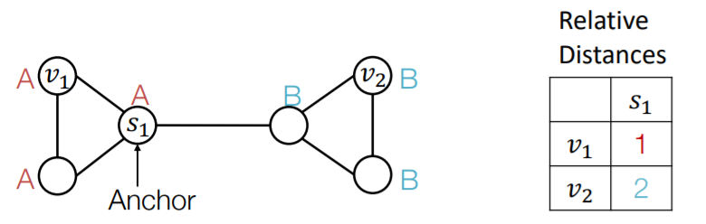
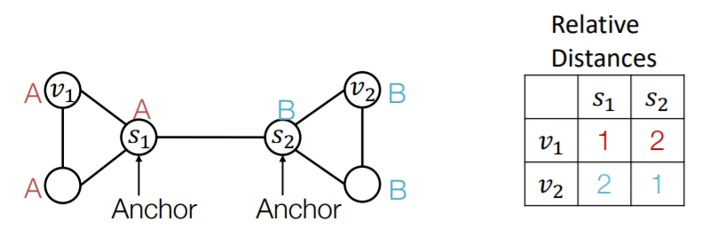
(3) Anchor

a) Anchor node

• randomly pick node \(s_1\) as “anchor node”

• represent \(v_1\) & \(v_2\) with “relative distances w.r.t \(s_1\)“

  ( = act as “coordinate axis” )

b) Multiple anchor nodes

• randomly pick node \(s_1\) & \(s_2\) as “anchor nodes”
• more anchors ( = many coordinate axes ) \(\rightarrow\) better characterization

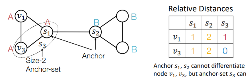
c) Anchor-sets

• ( generalization ) single node \(\rightarrow\) set of nodes
• can save the total number of anchors

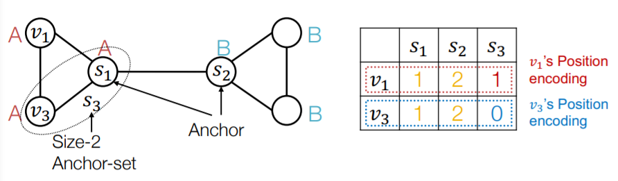
d) Summary

• can see it as “position encoding”
  • represent node’s position, by using “distance from anchor-sets”
• use this as “augmented node feature”
• need NN that can maintain “permutation invariant property of PE”

3. Identity-aware GNN

GNN

• fail for position-aware task
• but, still not perfect for structure-aware tasks!
• failure
  • 1) node-level
  • 2) edge-level
  • 3) graph-level

(1) Problems

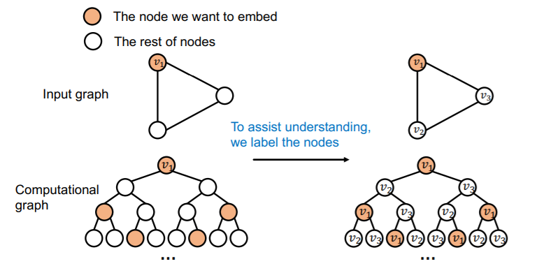
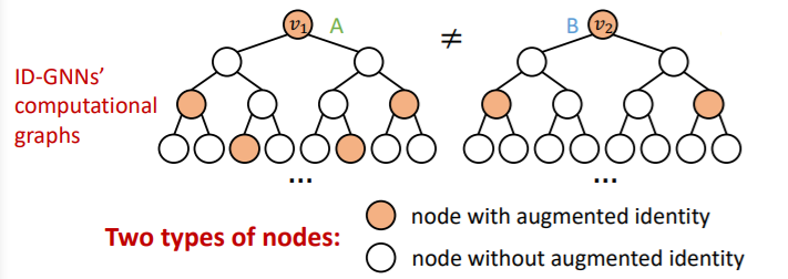
(a) failure in Node-level Tasks

problem ) DIFFERENT input, SAME computational graph

(b) failure in Edge-level Tasks

problem ) DIFFERENT input, SAME computational graph

( of course, because “edge” depends on “two nodes” )

(c) failure in Graph-level Tasks

problem ) DIFFERENT input, SAME computational graph

if we draw 2-hop computational graphs…

(2) Solution : Inductive Node Coloring

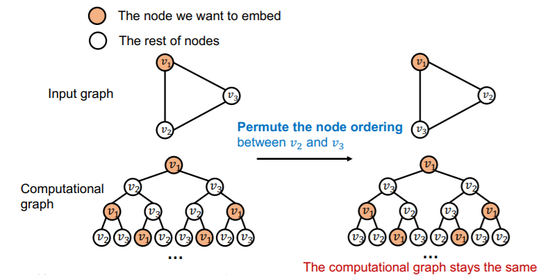
key idea : color the target node (that we want to embed)

Coloring is “Inductive”

( = invariant to node order/identities )

a) node-level

ex) node classification

• Input graphs :

  

• Computational graphs : different!

  

b) graph-level

ex) graph classification

• Input graphs :

  

• Computational graphs : different!

  

c) edge-level

ex) link prediction

• Input graphs :

  

• Computational graphs : different!

  

Link-prediction = “classifying a pair of nodes”

• step 1) color one of the node ( \(v_0\) )
• step 2) embed the other node ( \(v_1\) or \(v_2\) )
• step 3) use “node embedding of \(v_1\) (or \(v_2\))”, conditioned on \(v_0\)

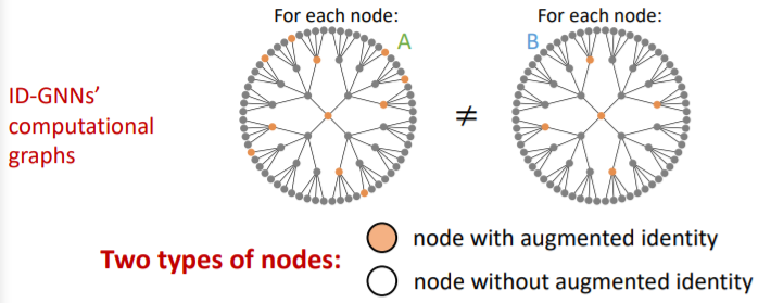
(3) Identity-aware GNN ( ID-GNN )

key point : use inductive node coloring

\(\rightarrow\) heterogenous message passing

( = different message passing to different nodes )

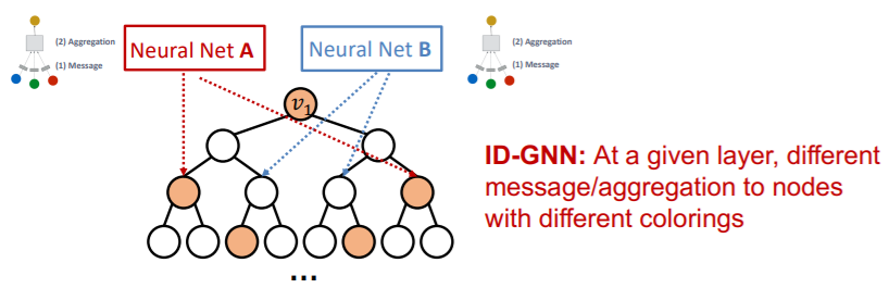
Thus, it will have “different embedding” !

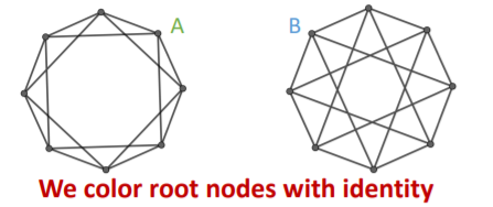
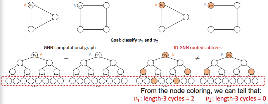
GNN vs ID-GNN

Comparison

• GNN : can NOT count cycles, originating from a given node
• ID- GNN : can count cycles, originating from a given node

( Left : GNN & Right : ID-GNN )

(4) ID-GNN-Fast

ID-GNN-Fast = Simple version of ID-GNN

Comparison

• ID-GNN : heterogenous MP (O)

• ID-GNN-Fast : heterogenous MP (X)

  • rather, use identity information as augmented node feature

    ( e.g. use “cycle counts”)

(5) Summary of ID-GNN

General & Powerful extension to GNN framework

• applicable to “any message passing GNNs”
• more expressive than original GNN ( 1-WL test )
• can easily implement ( PyG, DGL )

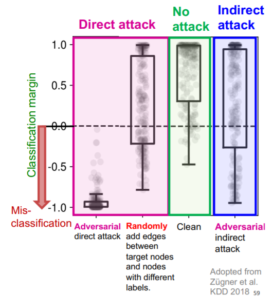
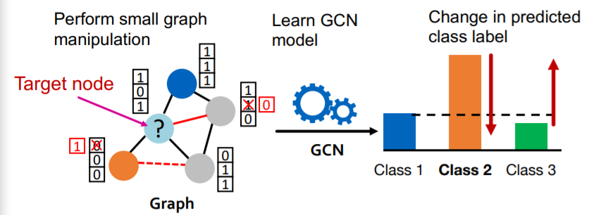
4. Robustness of GNN

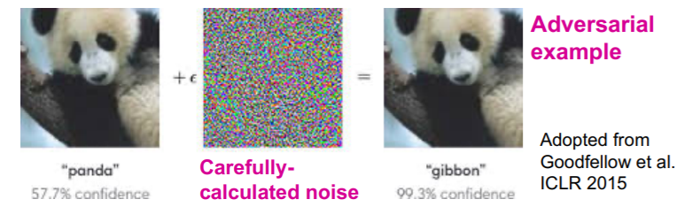
(1) Adversarial attacks

small perturbation on data, huge difference in output!

Problem )

• prevents the reliable deployment of DL models to real world

example )

(2) Settings

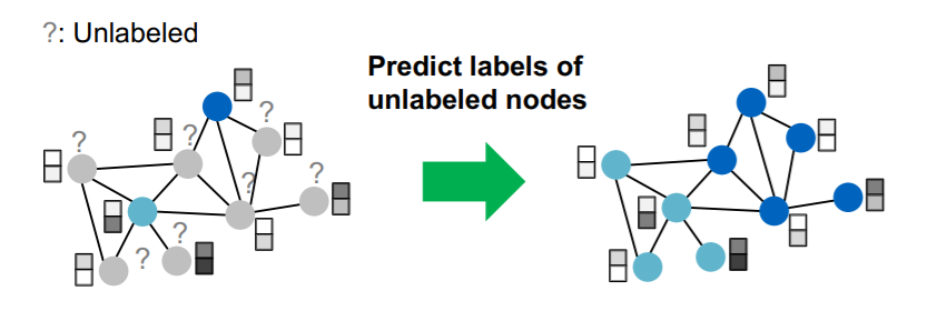
• Task : semi-supervised node classification

• Model : GCN

Concepts

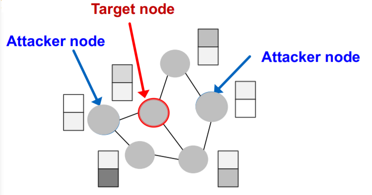
• Target node \(t \in V\)

  • node to be attacked

    ( = want to change “label prediction” )

• Attacker nodes \(S \in V\)

  • nodes, that attacker can modify

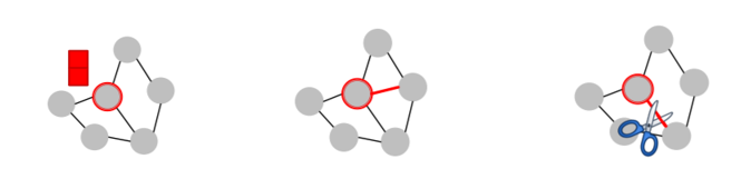
(3) Attack possibilities

a) Direct attack

• attacker node = target node ( \(S = \{t\}\) )
• 3 types
  • 1) modify target “node feature”
  • 2) “add connection” to target
  • 3) “remove connection” from target

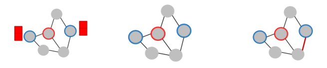
b) Indirect attack

• attacker node \(\neq\) target node ( \(t \notin S\) )

• 3 types

  • 1) modify attacker “node feature”
  • 2) “add connection” to attacker
  • 3) “remove connection” from attacker

(4) Goal of attacker

MAXIMIZE “change of target node label prediction”

• SUBJECT TO “small graph manipulation”

(5) Mathematical Formulation

Notation

• Original graph

  • \(\boldsymbol{A}\) : adjacency matrix
  • \(\boldsymbol{X}\) : feature matrix

• Manipulated graph ( with noise )

  • \(\boldsymbol{A}'\) : adjacency matrix
  • \(\boldsymbol{X}'\) : feature matrix

• Assumption : \(\left(\boldsymbol{A}^{\prime}, \boldsymbol{X}^{\prime}\right) \approx(\boldsymbol{A}, \boldsymbol{X})\)

  • meaning = “small” graph manipulation

    ( preserve basic graph/feature statistics )

• Target node : \(v \in V\)

Graph manipulation : can be both

• 1) direct
• 2) indirect

ORIGINAL graph

• parameter of GCN ( with ‘original graph’ )

  • \(\boldsymbol{\theta}^{*}=\operatorname{argmin}_{\boldsymbol{\theta}} \mathcal{L}_{\text {train }}(\boldsymbol{\theta} ; \boldsymbol{A}, \boldsymbol{X})\).

• prediction of GCN ( on ‘target node’ )

  • \(c_{v}^{*}=\operatorname{argmax}_{c} f_{\theta^{*}}(A, X)_{v, c}\).

  ( = predicted class of node \(v\) )

MANIPULATED graph

• parameter of GCN ( with ‘manipulated graph’ )

  • \(\boldsymbol{\theta}^{* \prime}=\operatorname{argmin}_{\boldsymbol{\theta}} \mathcal{L}_{\text {train }}\left(\boldsymbol{\theta} ; \boldsymbol{A}^{\prime}, \boldsymbol{X}^{\prime}\right)\).

• prediction of GCN ( on ‘target node’ )

  • \(c_{v}^{* \prime}=\operatorname{argmax}_{c} f_{\theta^{* \prime}}\left(A^{\prime}, X^{\prime}\right)_{v, c}\).

  ( = predicted class of node \(v\) )

Goal : \(c_{v}^{* \prime} \neq c_{v}^{*}\)

• change the prediction after manipulation!

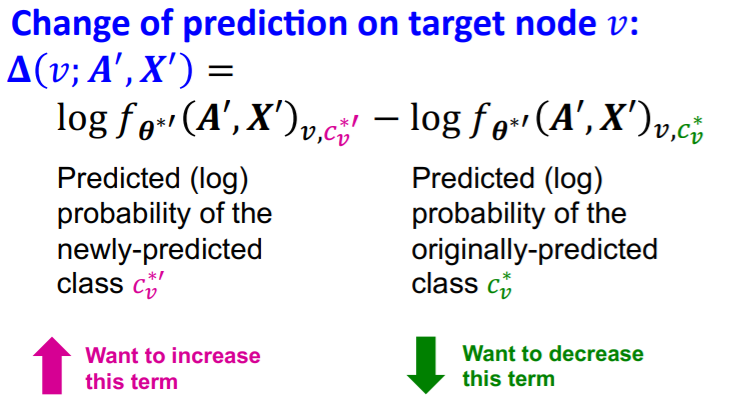
Optimization

• \(\operatorname{argmax}_{A^{\prime}, X^{\prime}} \Delta\left(v ; \boldsymbol{A}^{\prime}, \boldsymbol{X}^{\prime}\right)\),

  subject to \((\boldsymbol{A}^{\prime}, \boldsymbol{X}^{\prime}) \approx (\boldsymbol{A}, \boldsymbol{X})\)

• problem :

  • 1) \(\boldsymbol{A}^{'}\) is discrete

  • 2) for every modified \(\boldsymbol{A}^{'}\) & \(\boldsymbol{X}^{'}\),

    need to be “re-trained” ( computationally expensive )

(6) Experiments

Power of attack

• (1) Direct > (2) Indirect > (3) Random attack