(CS224W) 2.Traditional Methods for ML on Graphs

[ 2. Traditional Methods for ML on Graphs ]

( 참고 : CS224W: Machine Learning with Graphs )

Contents

• 2-1. Traditional Feature-based Methods : Node
• 2-2. Traditional Feature-based Methods : Link
• 2-3. Traditional Feature-based Methods : Graph

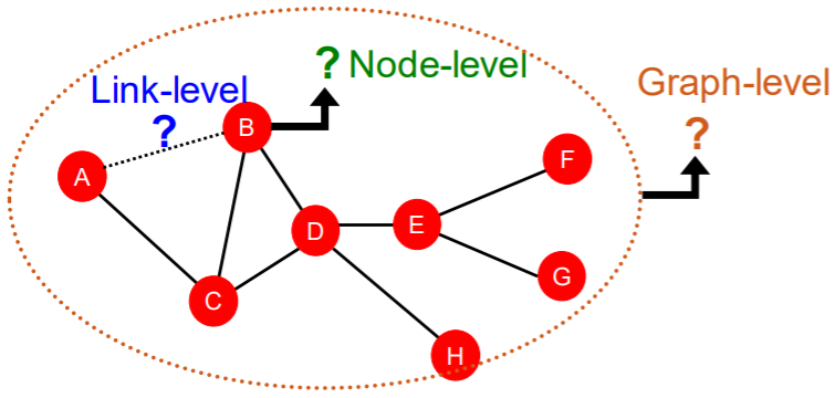
ML tasks with graph

• Node-level prediction
• Link-level prediction
• Graph-level prediction

Traditional ML Pipeline

• design “node features”,”link features”,”graph features”

  ( traditional method : “hand-designed” features )

• 2 steps

  • Step 1 : train an ML model

  • Step 2 : apply the model

( will focus on undirected graphs for simplicity )

Goal : make “prediction” for node/link/graph

Design choices

• features : \(d\)-dim vector
• objects : node / edge / set of nodes / graph
• objective functions

2-1. Traditional Feature-based Methods : Node

1) Node-level tasks

ex) Node classification

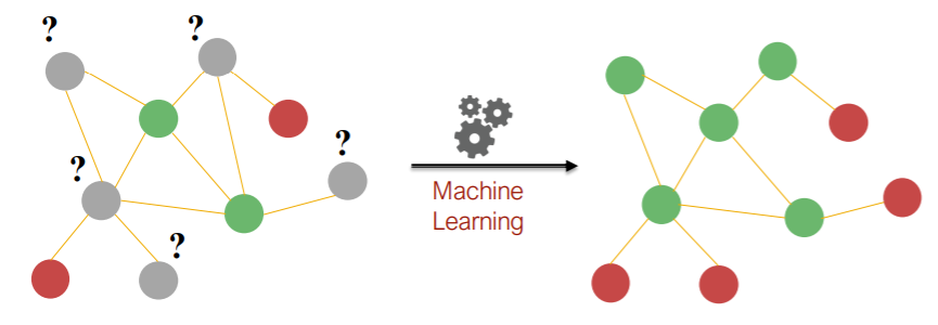
Goal : characterize “node” in structure

• 1) node degree
• 2) node centrality
• 3) clustering coefficient
• 4) graphlets

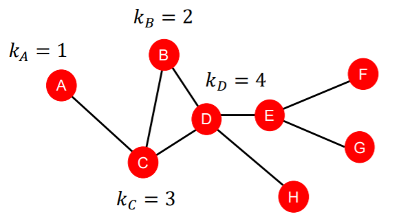
1) Node Degree

• \(k_v\) : number of edges in node \(v\)
• simple, but very useful feature!
• treat all neighbors equally

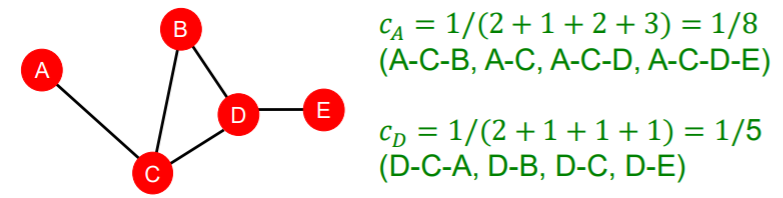
2) Node Centrality

Problems of node degree :

• do not consider nodes’ importance

  \(\rightarrow\) use “Node Centrality”

Node centrality

• \(c_v\): importance of node \(v\) in a graph
• example
  • 1) eigenvector centrality
  • 2) betweenness ~
  • 3) closeness ~

(a) Eigenvector centrality

important, if it is surrounded by important nodes

\(c_{v}=\frac{1}{\lambda} \sum_{u \in N(v)} c_{u}\) \(\leftrightarrow\) \(\lambda c = Ac\)

• \(\lambda\) : positive constant
• \(A\) : adjacency matrix
• \(c\) : centrality vector

leading eigenvector \(c_{max}\) is used for centrality

(b) Betweenness centrality

important, if it lies in the shortest path between 2 nodes

\(c_{v}=\sum_{s \neq v \neq t} \frac{\#(\text { shortest paths betwen } s \text { and } t \text { that contain } v)}{\#(\text { shortest paths between } s \text { and } t)}\).

(c) Closeness centrality

important, if it has small shortest path lengths to all other nodes

\(c_{v}=\frac{1}{\sum_{u \neq v} \text { shortest path length between } u \text { and } v}\).

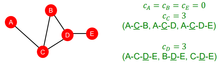
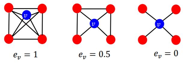
3) Clustering Coefficients

measure how connected node \(v\)’s NEIGHBORS are!

\(e_{v}=\frac{\#(\text { edges among neighboring nodes })}{\left(\begin{array}{c} k_{v} \\ 2 \end{array}\right)} \in[0,1]\).

• \(\left(\begin{array}{c} k_{v} \\ 2 \end{array}\right)\) : # of node pairs, among \(k_v\) neighboring nodes

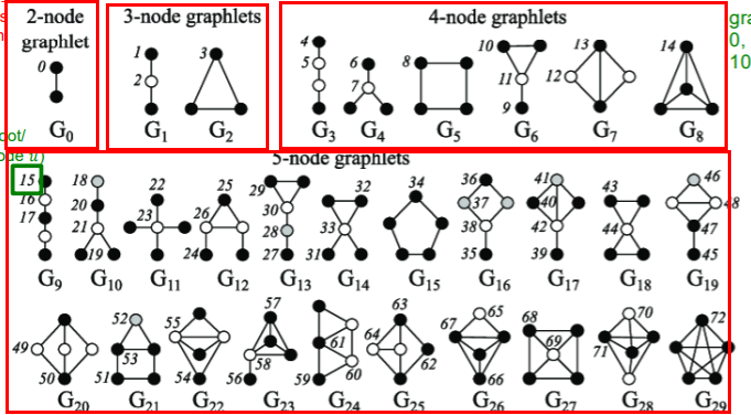
4) Graphlets

clustering coefficients :

• count the # of triangles in the ego-network

\(\rightarrow\) generalize, by counting graphlets

( graphlets : rooted connected non-isomorphic subgraphs )

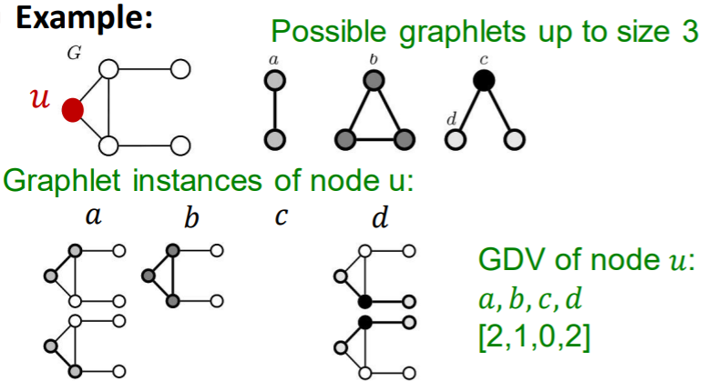
Definition

• GDV (Graphlet Degree Vector) :
  • graphlet-base features for nodes
  • # of graphlets that node touches
• Degree :
  • # of edges that node touches
• Clustering Coefficients
  • # of triangles that node touches

Summary

• importance-based features :
  • 1) node degree
  • 2) node centrality measures
    • eigenvector / betweenness / closeness centrality
• structure-based features :
  • 1) node degree
  • 2) clustering coefficients
    • how connected neighbors are to each other
  • 3) graphlet degree vector
    • occurences of different graphlets

2-2. Traditional Feature-based Methods : Link

predict “new links”

( whether 2 nodes are connected! )

Key point : how to design features for PAIR OF NODES

1) Two formulations of link prediction

• 1) Links Missing At Random

  • step 1) remove random set of links
  • step 2) predict them

• 2) Links over time

  • network that changes over time!

  • input : \(G[t_0, t_0']\)

    ( = graphs, up to time \(t_o'\) )

  • output : ranked list \(L\) of links

    ( that are not in \(G[t_0, t_0']\), but is predicted to appear in \(G[t_1, t_1']\) )

2) Link prediction, via Proximity

notation

• pair of nodes : \((x,y)\)
• score of \((x,y)\) : \(c(x,y)\)
  • ex) # of common neighbors of \(x\) and \(y\)

Step 1) Sort “pair of nodes”, by their “score” ( decreasing order )

Step 2) Predict top \(n\) pairs, as new links

3) Link feature

• distance-based feature
• local neighborhood overlap
• global neighborhood overlap

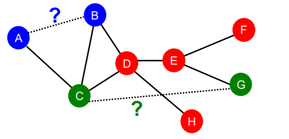
(a) distance based feature

• shortest-path distance between 2 nodes
• problem
  • does not capture “degree of neighborhood of overlap”

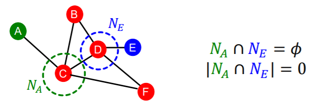
(b) local neighborhood overlap

• # of neighboring nodes, shared between 2 nodes
• example
  • 1) common neighbors : \(\mid N\left(v_{1}\right) \cap N\left(v_{2}\right) \mid\)
  • 2) Jaccard’s coefficient : \(\frac{ \mid N\left(v_{1}\right) \cap N\left(v_{2}\right) \mid }{ \mid N\left(v_{1}\right) \cup N\left(v_{2}\right) \mid }\)
  • 3) Adamic-Adar index : \(\sum_{u \in N\left(v_{1}\right) \cap N\left(v_{2}\right)} \frac{1}{\log \left(k_{u}\right)}\)
    • \(k_u\) : degree of node \(u\)
    • consider neighbor’s importance by its degree

Limitation :

• zero, when 2 nodes don’t share any nodes

  ( but may have potential to be connected! )

• thus, use GLOBAL neighborhood overlap

  ( by considering “ENTIRE” graph )

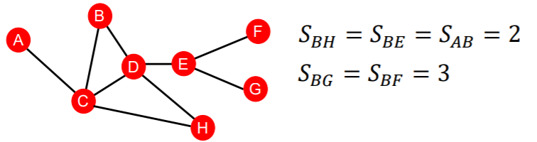
(c) global neighborhood overlap

(intro) Katz index

• # of paths of all lengths between 2 nodes
• how? by calculating “Powers of graph Adjacency Matrix”
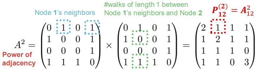
• Theory
  • \(\boldsymbol{P}_{u v}^{(K)}\) = # of paths of length \(\boldsymbol{K}\) between \(\boldsymbol{u}\) and \(\boldsymbol{v}\)
  • \(P^{(K)}=A^{k}\).
• ex) \(A^2_{uv}\) : # of paths of length 2, between \(u\) & \(v\)

Katz index

• sum over all path lengths

• \(S_{v_{1} v_{2}}=\sum_{l=1}^{\infty} \beta^{l} \boldsymbol{A}_{v_{1} v_{2}}^{l}\).
  • \(\beta\) : discount factor
  • \(\boldsymbol{A}_{v_{1} v_{2}}^{l}\) : # paths of length \(l\), between \(v_1\) & \(v_2\)
• closed form solution :
  • \(\boldsymbol{S}=\sum_{i=1}^{\infty} \beta^{i} \boldsymbol{A}^{i}=\underbrace{(\boldsymbol{I}-\beta \boldsymbol{A})^{-1}}_{=\sum_{i=0}^{\infty} \beta^{i} A^{i}}-\boldsymbol{I}\).

2-3. Traditional Feature-based Methods : Graph

Goal : want feature that considers structure of ENTIRE GRAPH

\(\rightarrow\) use Kernel Methods

1) Kernel Methods

Key Idea :

• design “kernels”, instead of “feature vectors”

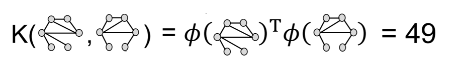
Kernel & Kernel matrix

• kernel \(K(G,G')\) : similarity between data
  • \[K(G,G') = \phi(G)^T\phi(G')\]
• kernel matrix \(K=(K(G,G'))_{G,G'}\) : positive semi-definite

2) Graph kernels

measures similarity between 2 graphs

• 1) Graphlet Kernel
• 2) Weisfeiler-Lehman Kernel

Goal : design graph feature vector \(\phi(G)\)

Key Idea : BoW( + \(\alpha\) ) for a graph

(1) simple version : Bag-of-Words

• just treat node as words

• example )

  

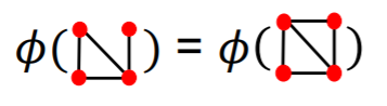
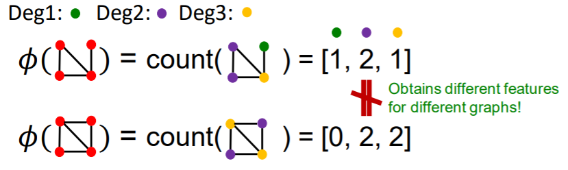
(2) Bag-of-“Node degrees”

• example )

  

Graphlet Kernel & Weisfeiler-Lehman Kernel

\(\rightarrow\) both uses “Bag-of-xx” concept!

3) Graphlet Kernel

• # of different graphlets in a graph
• Node-level vs Graph-level
  • (1) do not need to be connected
  • (2) are not rooted
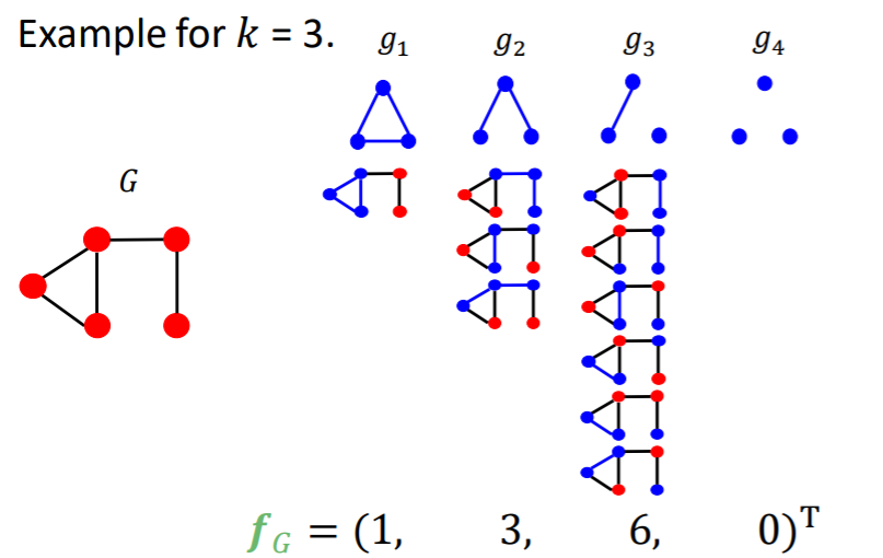
  • example)

Notation

• \(G\) : graph
• \(G_k = (g_1,..,g_{n_k})\) : graphlet list
• \(f_g \in R^{n_k}\) : graphlet count vector
  • \(\left(\boldsymbol{f}_{G}\right)_{i}=\#\left(g_{i} \subseteq G\right) \text { for } i=1,2, \ldots, n_{k}\).
• \(K(G,G') = f_G^T f_{G'}\) : graphlet kernel
• 

Problem

• if size of \(G\) & \(G'\) is different…. skew the value

Solution

• normalize each feature vector
• \(K\left(G, G^{\prime}\right)=\boldsymbol{h}_{G}{ }^{\mathrm{T}} \boldsymbol{h}_{G^{\prime}}\).
  • where \(\boldsymbol{h}_{G}=\frac{\boldsymbol{f}_{G}}{\operatorname{Sum}\left(\boldsymbol{f}_{G}\right)}\).

Limitation

• too expensive to count graphlets!

• how to design more efficient kernel?

  \(\rightarrow\) Weisfeiler-Lehman Kernel

4) Weisfeiler-Lehman Kernel

Goal :

• design an “EFFICIENT” graph feature descriptor \(\phi(G)\)

Key Idea

• use neighborhood structure to iteratively enrich node vocabulary
• ( = generalized version of Bag of “node-degrees” )

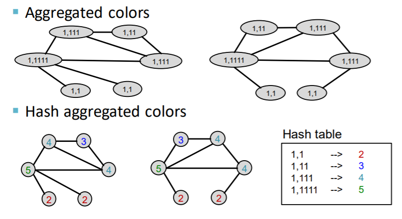
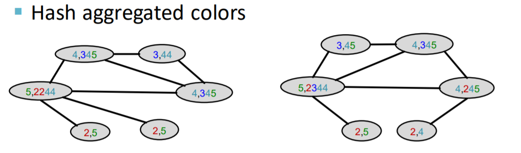
Algorithm : COLOR REFINEMENT

Color Refinement

• (notation) graph \(G\) with nodes \(V\)

• process

  • step 1) assign initial color \(c^{(0)}(v)\) to each node \(v\)

  • step 2) iteratively refine node colors…..

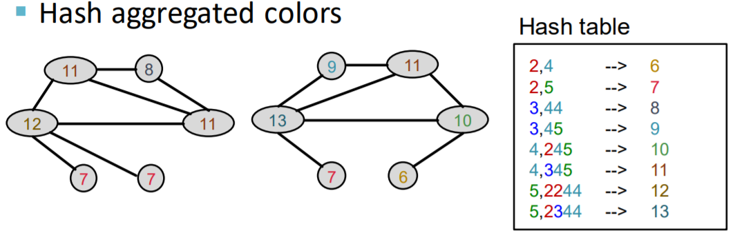
    • \(C^{(k+1)}(v)=\operatorname{HASH}\left(\left\{C^{(k)}(v),\left\{C^{(k)}(u)\right\}_{u \in N(v)}\right\}\right)\).

    • HASH : mapping function

      ( different input to different color )

  • ….

  • after \(K\) steps of color refinement,

    \(c^{(K)}(v)\) : structure of \(K\)-hop neighborhood

5) Summary of graph kernels

Graphlet Kernel

• summary
  • graph = “bag of GRAPHLETS”
• disadvantage
  • computationally expensive

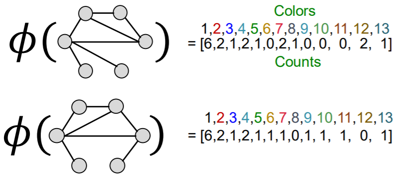
Weisfeiler-Lehman Kernel

• summary
  • apply \(K\)-step color refinement
  • graph = “bag-of-COLORS”
  • closely related to GNN
• advantages

  • computationally efficient

  • only colors need to be tracked

    \(\rightarrow\) # of colors : at most # of nodes

  • time complexity : linear in # of edges

Summary

Traditional ML

• hand-made feature + ML model

Hand-made features :

• 1) node-level
  • node degree
  • node centrality
  • clustering coefficients
  • graphlets
• 2) link-level
  • distance-based feature
  • local & global neighborhood overlap
• 3) graph-level
  • graphlet kernel
  • WL kernel