(CS224W) 3.Node Embedding

[ 3. Node Embedding ]

( 참고 : CS224W: Machine Learning with Graphs )

Contents

• 3-1. Node Embeddings
• 3-2. Random Walk
• 3-3. Embedding Entire Graphs

3-1. Node Embeddings

1) Feature Representation ( Embedding )

Goal : create an…

• 1) efficient
• 2) task-independent feature learning
• 3) with graphs!

Similar in Network \(\approx\) Similar in Embedding Space

With these embeddings…solve many tasks!

• ex) node classification, link prediction….

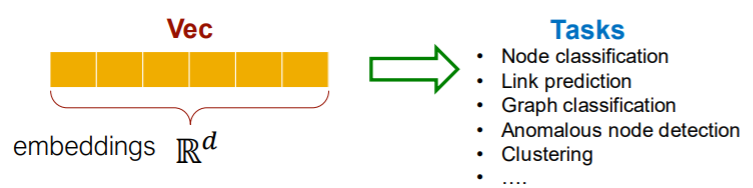
Node Embedding algorithms

• ex) Deep Walk

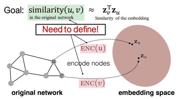
2) Encoder & Decoder

Notation

• graph \(G\)
• vertex set \(V\)
• adjacency matrix \(A\) ( binary )

Goal : encode nodes, such that….

“similarity in embedding space \(\approx\) similarity in graph”

( \(\operatorname{similarity}(u, v) \approx \mathbf{z}_{v}^{\mathrm{T}} \mathbf{z}_{u}\) )

key point : how do we DEFINE SIMILARITY??

Process

• step 1) node —-(encoder)——> embeddings

  ( \(\operatorname{ENC}(v)=\mathbf{z}_{v}\) )

• step 2) define “node similarity function”

• step 3) embedding—–(decoder)——> similarity score

• step 4) optimization

  ( in a way that \(\operatorname{similarity}(u, v) \approx \mathbf{z}_{v}^{\mathrm{T}} \mathbf{z}_{u}\) )

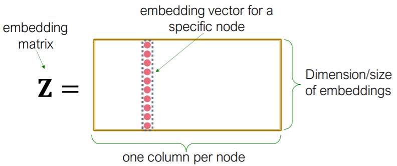
3) Shallow Encoding

• simplest ( just “embedding-lookup table” )
• \(\operatorname{ENC}(v)=\mathbf{z}_{v}=\mathbf{Z} \cdot v\).
  • where \(\mathbf{Z} \in \mathbb{R}^{d \times \mid \mathcal{V} \mid }\) ( what we want to learn )
  • \(v \in \mathbb{I}^{ \mid \mathcal{V} \mid }\) : indicator vector
• ex) Deep Walk, node2vec

4) How to define “Node Similarity”?

candidates : does/are 2 nodes…

• are linked?
• share neighbors?
• have similar roles in graph ( = structural roles )?

\(\rightarrow\) will learn “node similarity” that uses random walks!

Notes

• unsupervised / self-supervised tasks
  • node labels (X), node features (X)
• these embeddings are “task independent”

3-2. Random Walk

1) Introduction

Notation

• \(z_u\) : embedding of \(u\)
• \(P(v \mid z_u)\) : (predicted) probability of visiting \(v\), starting from \(u\) ( on random walks )
• \(R\) : random walk strategy

Random Walk

• start from arbitrary node
• move to adjacent(neighbor) nodes RANDOMLY
• Random Walk : “sequence of points visited” in this way
• \(z^T_u z_v\) \(\approx\) probability that \(u\) & \(v\) co-occur on random walk
• nearby nodes : via \(N_R(u)\)
  • neighborhood of \(u\), obtained by strategy \(R\)

2) Random Walk Embeddings

Random Walk Embeddings

• step 1) estimate \(P_R(v \mid u)\)
• step 2) optimize embeddings, to encode these random walk statistics
  • cosine similarity \((z_i, z_j)\) \(\propto P_R(v \mid u)\)

Advantages of Random Walk

• 1) Expressivity

  • captures both local & higher-order neighborhood info

• 2) Efficiency

  • do not consider ALL nodes

    ( only consider “PAIRS” that co-occur in random walk )

Feature Learning as Optimization

• goal :
  • learn \(f(u) = z_u\)
• objective function :
  • \(\max _{f} \sum_{u \in V} \log \mathrm{P}\left(N_{\mathrm{R}}(u) \mid \mathbf{z}_{u}\right)\).

3) Procedure

• step 1) Run short fixed-length random walk

  • starting node : \(u\)
  • random walk strategy : \(R\)

• step 2) collect \(N_R(u)\)

  • ( = multiset of nodes visited )

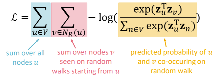
• step 3) optimize embedding

  • \(\max _{f} \sum_{u \in V} \log \mathrm{P}\left(N_{\mathrm{R}}(u) \mid \mathbf{z}_{u}\right)\).

    ( equivalently, \(\mathcal{L}=\sum_{u \in V} \sum_{v \in N_{R}(u)}-\log \left(P\left(v \mid \mathbf{z}_{u}\right)\right)\) )

  • \(P\left(v \mid \mathbf{z}_{u}\right)\) : parameterize as softmax

    \(\rightarrow\) but TOO EXPENSIVE ( \(O(\mid V \mid^2)\) )… let’s approximate it

    via NEGATIVE SAMPLING

4) Negative Sampling

\(\log \left(\frac{\exp \left(\mathbf{z}_{u}^{\mathrm{T}} \mathbf{z}_{v}\right)}{\sum_{n \in V} \exp \left(\mathbf{z}_{u}^{\mathrm{T}} \mathbf{z}_{n}\right)}\right) \approx \log \left(\sigma\left(\mathbf{z}_{u}^{\mathrm{T}} \mathbf{z}_{v}\right)\right)-\sum_{i=1}^{k} \log \left(\sigma\left(\mathbf{z}_{u}^{\mathrm{T}} \mathbf{z}_{n_{i}}\right)\right), n_{i} \sim P_{V}\).

• do not use all nodes

  only some “negative samples” \(n_i\)

  ( sampled not uniformly, but in a biased way )

• biased way = “proportional to its degree”

• appropriate \(k\)

  • higher \(k\) : more robust & higher bias on negative events
  • in practice, \(k=5 \sim 20\)
  • optimize using SGD

5) Strategies of walking

• example) Deep Walk
• how to generalize?? “node2vec”

node2vec

• key point : biased 2nd order random walk to generate \(N_R(u)\)
• https://seunghan96.github.io/ne/ppt/4.node2vec/

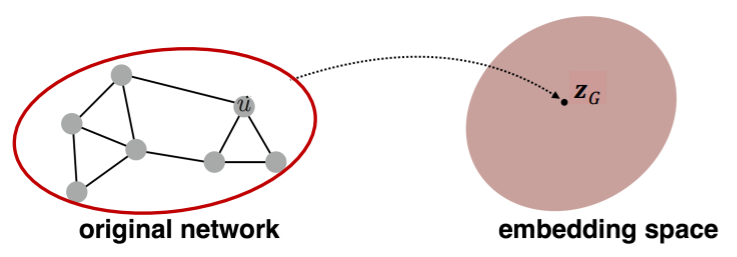
3-3. Embedding Entire Graphs

ex) classify toxic/non-toxic molecules

1) Idea 1 (simple)

• standard graph embedding
• sum the node embeddings in the graph
• \(\boldsymbol{z}_{\boldsymbol{G}}=\sum_{v \in G} Z_{v}\).

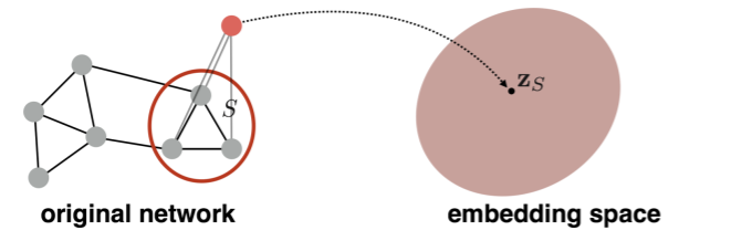
2) Idea 2

• use “virtual node”
• this node will represent the entire graph!

3) Idea 3 ( Anonymous Walk Embeddings )

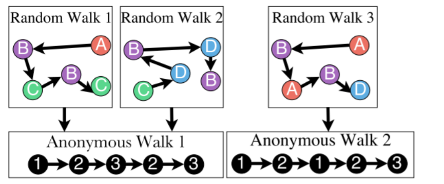
• do not consider which specific node it visisted!
  • = agnostic to the identity
  • = anonymous
• # of anonymous walks grows exponentially
• ex) \(l=3\)
  • 5-dim representation
  • 111,112,121,122,123
  • \(Z_G[i]\) = prob of anonymous walk \(w_i\) in \(G\)
• sampling anonymous walks
  • generate \(m\) random walks
  • appropriate \(m\) ?
    • \(m=\left[\frac{2}{\varepsilon^{2}}\left(\log \left(2^{\eta}-2\right)-\log (\delta)\right)\right]\).
      • \(\eta\) : # of anonymous walks of length \(l\)

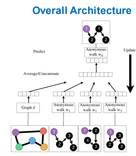
Learn Embeddings

• learn \(z_i\) ( = embedding of walk \(w_i\) )

• learn \(Z_G\) ( = graph embedding, \(Z=\left\{z_{i}: i=1 \ldots \eta\right\}\) )

• how to embed walks?

  • learn to predict walks, that co-occur in \(\Delta\) size window

  • \(\max \sum_{t=\Delta}^{T-\Delta} \log P\left(w_{t} \mid w_{t-\Delta}, \ldots, w_{t+\Delta}, z_{G}\right)\).

    \(\rightarrow\) sum the objective, over ALL nodes

Process

• step 1) run \(T\) different random walks, of length \(l\)
  • \(N_{R}(u)=\left\{w_{1}^{u}, w_{2}^{u} \ldots w_{T}^{u}\right\}\).
• step 2) optimize below
  • \(\max _{\mathrm{Z}, \mathrm{d}} \frac{1}{T} \sum_{t=\Delta}^{T-\Delta} \log P\left(w_{t} \mid\left\{w_{t-\Delta}, \ldots, w_{t+\Delta} \mathbf{z}_{\boldsymbol{G}}\right\}\right)\).
    • \(P\left(w_{t} \mid\left\{w_{t-\Delta}, \ldots, w_{t+\Delta}, z_{G}\right\}\right)=\frac{\exp \left(y\left(w_{t}\right)\right)}{\sum_{i=1}^{\eta} \exp \left(y\left(w_{i}\right)\right)}\).
    • \(y\left(w_{t}\right)=b+U \cdot\left(\operatorname{cat}\left(\frac{1}{\Delta} \sum_{i=1}^{\Delta} \mathbf{z}_{i}, \mathbf{z}_{G}\right)\right)\).
      • \(\operatorname{cat}\left(\frac{1}{\Delta} \sum_{i=1}^{\Delta} \mathbf{z}_{i}, \mathbf{z}_{G}\right)\) : avg of walk embeddings in the window, concatenated with graph embedding
  • just treat $z_G$ like $z_i$, when optimizing!
• step 3) obtain graph embedding \(Z_G\)

4) How to use embeddings

by using embeddings of nodes ( \(z_i\) )… we can solve…

• cluster/community detection
  • cluster nodes
• node classification
  • predict labels of nodes
• link prediction
  • predict edges of 2 nodes
  • how to use 2 node embeddings?
    • 1) concatenate
    • 2) Hadamard product
    • 3) sum / average
    • 4) distance
• graph classification
  • get graph embedding \(Z_G\), by aggregating node embeddings