(paper) Two-Stream(2s) AGCN for Skeleton-Based Action Recognition (2019)

Two-Stream(2s) AGCN for Skeleton-Based Action Recognition (2019)

Contents

1. Abstract
2. Introduction
3. Graph Convolution
4. Two-stream AGCN
   1. AGCN layer
   2. AGCN block
   3. AGCN

0. Abstract

Skeleton-based Action Recongition

• GCN is widely used!

• but, in existing GCN methods,

  • problem 1) topology of graph is set manually

  • problem 2) topology of graph is fixed over all layers & input

  \(\rightarrow\) may not be optimal for hierarchical GCN

proposes 2s-AGCN

( = Two Stream Adaptive GCN )

1. Introduction

Main Contributions

1. ADAPTIVE GCN is proposed,

   to adaptively learn the topology of the graph for different GCN layers & input samples

2. Second order info of skeleton data is explicitly formulated
3. propose 2s-AGCN

2. Graph Convolution

Graph Convolution Operation on \(v_i\) :

\(f_{\text {out }}\left(v_{i}\right)=\sum_{v_{j} \in \mathcal{B}_{i}} \frac{1}{Z_{i j}} f_{i n}\left(v_{j}\right) \cdot w\left(l_{i}\left(v_{j}\right)\right)\).

• \(f\) : feature map
• \(\mathcal{B}_{i}\) : sampling area of \(v_i\)

Implementation

Notation

• feature map : \(C \times T \times N\) tensor
• \(N\) : # of nodes
• \(T\) : temporal length
• \(C\) : # of channels

ST-GCN : \(\mathbf{f}_{o u t}=\sum_{k}^{K_{v}} \mathbf{W}_{k}\left(\mathbf{f}_{i n} \mathbf{A}_{k}\right) \odot \mathbf{M}_{k}\).

• \(K_{v}\) : kernel size of spatial dimension

• \(\mathbf{A}_{k}=\boldsymbol{\Lambda}_{k}^{-\frac{1}{2}} \overline{\mathbf{A}}_{k} \boldsymbol{\Lambda}_{k}^{-\frac{1}{2}}\).

  • \(\overline{\mathbf{A}}_{k}\) : similar to the \(N \times N\) adjacency matrix
    • \(\overline{\mathbf{A}}_{k}^{i j}\) : indicates whether the vertex \(v_{j}\) is in the subset \(S_{i k}\) of vertex \(v_{i}\)
  • \(\boldsymbol{\Lambda}_{k}^{i i}=\sum_{j}\left(\overline{\mathbf{A}}_{k}^{i j}\right)+\alpha\) : normalized diagonal matrix
    • \(\alpha\) is set to \(0.001\) to avoid empty rows.

• \(\mathbf{W}_{k}\) : \(C_{\text {out }} \times C_{i n} \times 1 \times 1\) weight vector ( 1x1 conv )

• \(\mathbf{M}_{k}\) : attention map

\(\rightarrow\) we perform a \(K_{t} \times 1\) convolution on the output feature map calculated above!

3. Two-stream AGCN

(1) AGCN layer

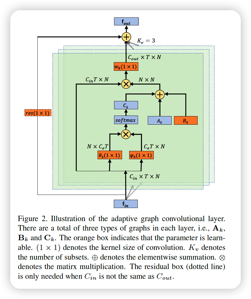
Notation

• \(\mathbf{A}_{k}\) : determines whether there are connections between two vertexes
• \(\mathbf{M}_{k}\) : determines the strength of the connections.

(BEFORE) \(\mathbf{f}_{o u t}=\sum_{k}^{K_{v}} \mathbf{W}_{k}\left(\mathbf{f}_{i n} \mathbf{A}_{k}\right) \odot \mathbf{M}_{k}\)

(AFTER) \(\mathbf{f}_{o u t}=\sum_{k}^{K_{v}} \mathbf{W}_{k} \mathbf{f}_{i n}\left(\mathbf{A}_{k}+\mathbf{B}_{k}+\mathbf{C}_{k}\right)\).

• to make it as an adaptive form

first part ( \(\mathbf{A}_{k}\) )

• original normalized \(N \times N\) adjacency matrix \(\mathbf{A}_{k}\)

second part \(\left(\mathbf{B}_{k}\right)\)

• \(N \times N\) adjacency matrix.

( in contrast to \(\mathbf{A}_{k}\), the elements of \(\mathbf{B}_{k}\) are parameterized and optimized ( data-driven ) )

• not only existence of connection, but also strength of connection
• play the same role of the attention, performed by \(\mathbf{M}_{k}\)
  • original attention. \(\mathbf{M_k}\) : dot multiplied to \(A_k\) …….. if zero, cannot generate new connections
  • thus, \(\mathbf{B_k}\) is more flexible!

third part \(\left(\mathbf{C}_{k}\right)\)

• data-dependent graph

  ( = unique graph for each sample )

• apply the normalized embedded Gaussian function to calculate the similarity of the two nodes

• \(f\left(v_{i}, v_{j}\right)=\frac{e^{\theta\left(v_{i}\right)^{T} \phi\left(v_{j}\right)}}{\sum_{j=1}^{N} e^{\theta\left(v_{i}\right)^{T} \phi\left(v_{j}\right)}}\).

• \(\mathbf{C}_{k}=\operatorname{softmax}\left(\mathbf{f}_{\mathbf{i n}}{ }^{T} \mathbf{W}_{\theta k}^{T} \mathbf{W}_{\phi k} \mathbf{f}_{\mathbf{i n}}\right)\).

  • where \(\mathbf{W}_{\theta}\) and \(\mathbf{W}_{\phi}\) are the parameters of the embedding functions

Summary

Rather than directly replacing the original \(\mathbf{A}_{k}\) with \(\mathbf{B}_{k}\) or \(\mathbf{C}_{k}\), we add them to it.

(2) AGCN block

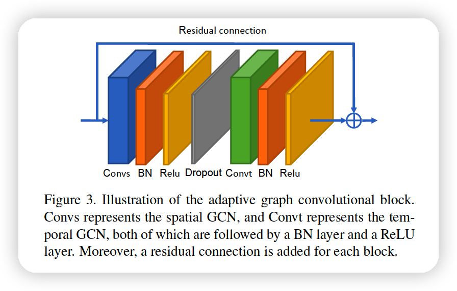
Convolution for TEMPORAL dimsneion

• \(K_{t} \times 1\) convolution on \(C \times T \times N\) feature maps

One block

• spatial GCN - BN - ReLU - DO - temporal GCN - BN - ReLU

• with Residual Connection

(3) AGCN

stack of AGCN blocks