(paper) GC-LSTM ; GCN embedded LSTM for Dynamic Network Link Prediction

GC-LSTM : GCN embedded LSTM for Dynamic Network Link Prediction (2018)

Contents

1. Abstract
2. Methodology
   1. Problem Definition
   2. Overall Framework
   3. GC-LSTM model
   4. Decoder Model
   5. Loss Function

0. Abstract

Dynamic Network Link Prediction

• challenge : network structure evolves with time

Propose GCN embedded LSTM ( = GC-LSTM ) for dynamic link prediction

• LSTM : for temporal features of all snapshots of dynamic network

• each snapshot : GCN is applied to capture local structural properties

• can predict both ADDED & REMOVED links
  • \(\leftrightarrow\) existing methods : only handle removed links

1. Methodology

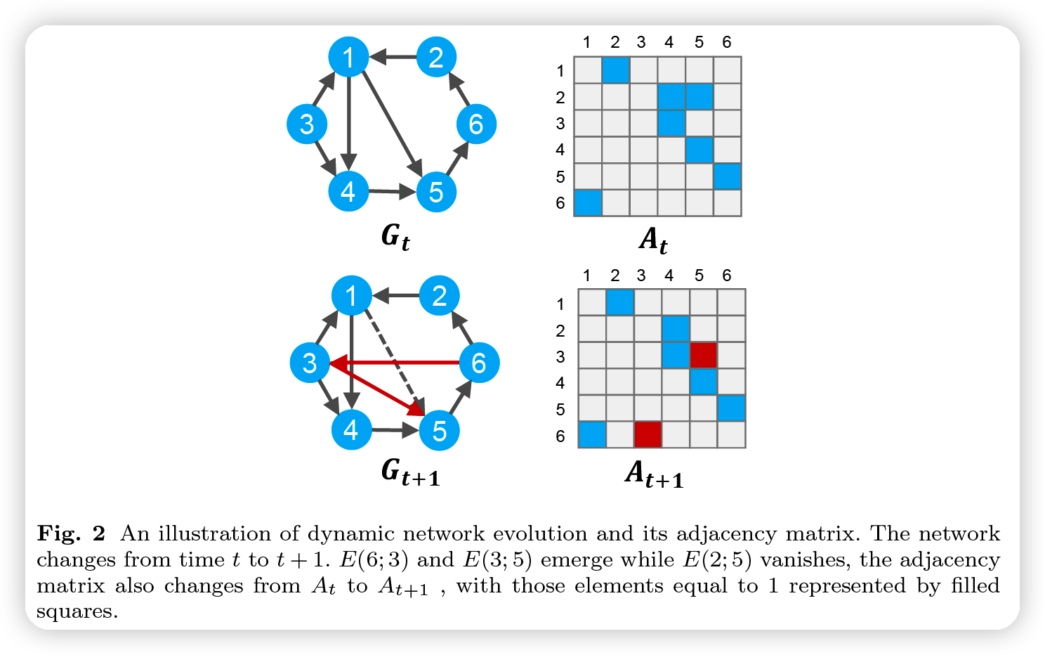
(1) Problem Definition

Dynamic Networks

sequence of discrete snapshots : \(\left\{G_{1}, \cdots, G_{T}\right\}\)

• \(G_{t}=\left(V, E_{t}, A_{t}\right)(t \in[1, T])\)……. network at time \(t\)
  • \(V\) : nodes
  • \(E_{t}\) : temporal links within the fixed timespan \([t-\tau, t]\)

Static Network

• aims to predict the future links by the current network

• focus on structural feature of the network

\(\leftrightarrow\) Dynamic network : also need to learn the temporal feature of the network

Goal

1. extract the structural feature of each snapshot network through GCN

2. learn temporal structure via LSTm

Network Link Prediction in Dynamic Networks

Dynamic network link prediction

• structural sequence modeling problem

• aims to learn the evolution information of the previous \(T\) snapshots,

  to predict the probability of all links at time t

• \(\hat{A}_{t}=\operatorname{argmax} P\left(A_{t} \mid A_{t-T}, \cdots, A_{t-1}\right)\).

(2) Overall Framework

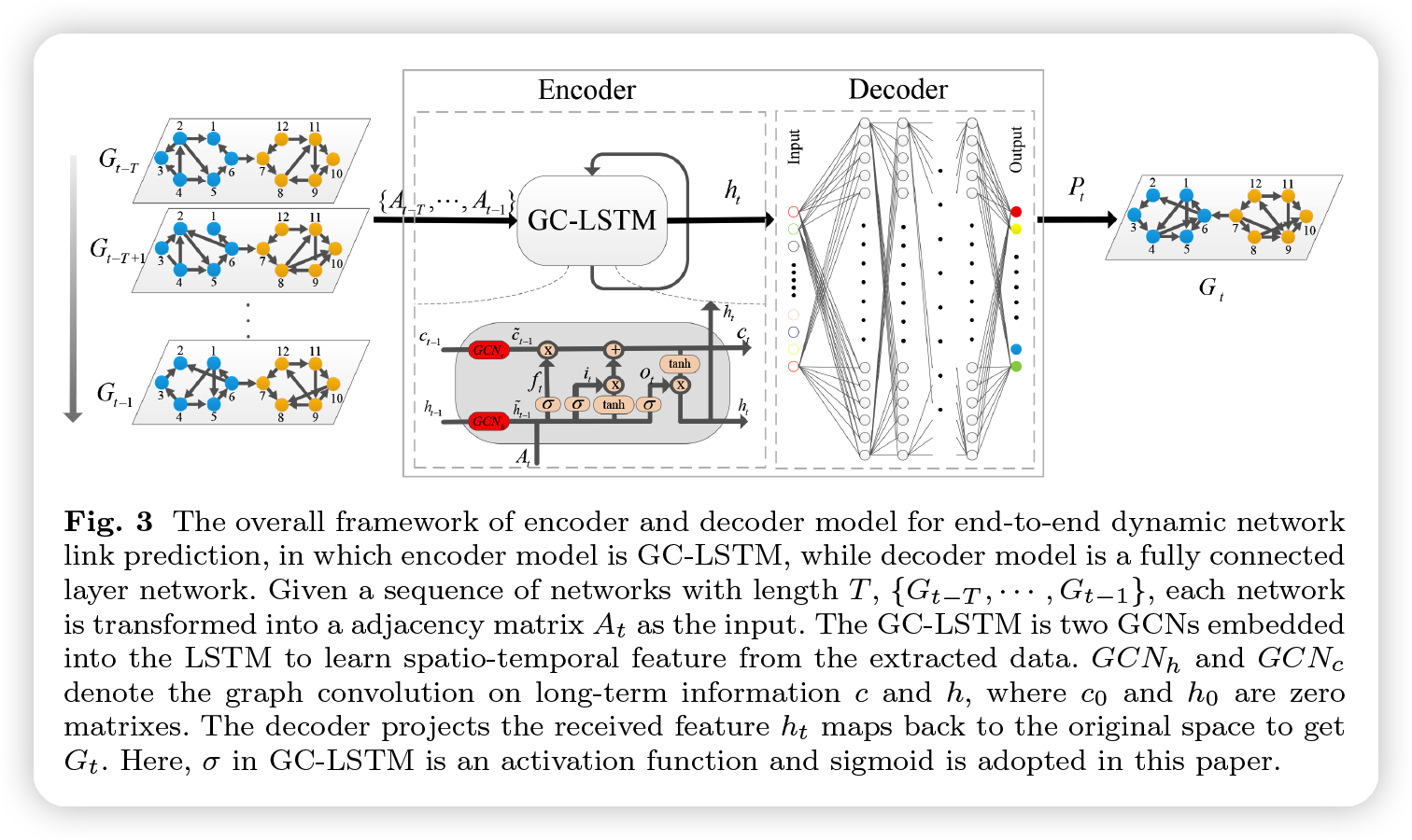
GC-LSTM

• encoder & decoder
• encoder = GCN embedded LSTM
  • GCN : learn network structure
  • LSTM : learn temporal information
• decoder = FC layer
  • convert feature map to original space

(3) GC-LSTM model

Input

• input sequence data : \(\left\{A_{t-T}, \cdots, A_{t-1}\right\}\)
• last hidden layer vector : \(h_{t}\)

Dynamic Network Link prediction

• linkage status of each node with others at multiple times

  = regarded as TIME SERIES

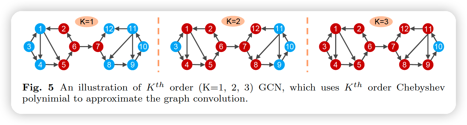
ChebNet : \(g_{\theta}=\sum_{k=0}^{K} \theta_{k} T_{k}(\tilde{L})\)

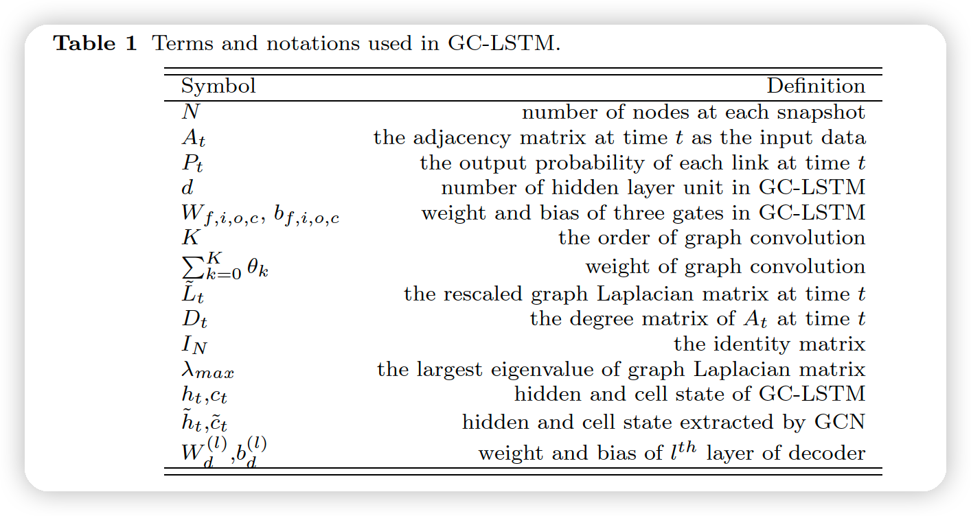
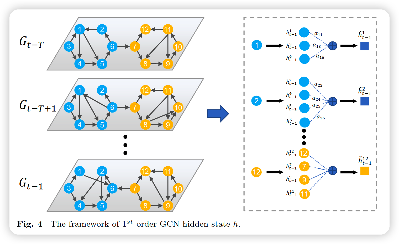
GC-LSTM model

• mainly relies on 2 state values

  • (1) hidden state \(h\)
  • cell state \(c\)

• in the dynamic network link prediction task,

  need to consider the influence of \(h\) of neighbors on \(h\) of target

  & influence of \(c\) of negibhros

\(\rightarrow\) thus, propose to use 2 GCN models, for \(h\) & \(c\)

Steps

[ step 1 ] Decide what info will be thrown away frm previous cell state

• by forget gate …… \(f_{t} \epsilon[0,1]^{d}\)
• \(f_{t}=\sigma\left(A_{t} W_{f}+G C N_{f}^{K}\left(\tilde{A}_{t-1}, h_{t-1}\right)+b_{f}\right)\).

[ Step 2 ] Update the cell state

• (1) \(\bar{c}_{t} \epsilon[-1,1]^{d}\) : tanh layer generates a new candidate vector of the cell layers,
• (2) \(i_{t} \epsilon[0,1]^{d}\) : sigmoid layer which determines how many new candidate vector will be added to the cell state
• (3) \(c_t\) : update cell state ( by (1) & (2) )

\(\begin{aligned} \bar{c}_{t} &=\tanh \left(A_{t} W_{c}+G C N_{o}^{K}\left(\tilde{A}_{t-1}, h_{t-1}\right)+b_{c}\right) \\ i_{t} &=\sigma\left(A_{t} W_{i}+G C N_{c}^{K}\left(\tilde{A}_{t-1}, h_{t-1}\right)+b_{i}\right) \\ c_{t} &=f_{t} \odot G C N_{c}^{K} c_{t-1}+i_{t} \cdot \bar{c}_{t} \end{aligned}\).

[ Step 3 ] Decide output ( by output gate )

\(\begin{aligned} &o_{t}=\sigma\left(A_{t} W_{o}+G C N_{o}^{K}\left(\tilde{A}_{t-1}, h_{t-1}\right)+b_{0}\right) \\ &h_{t}=o_{t} \odot \tanh \left(c_{t}\right) \end{aligned}\).

(4) Decoder model

\(\begin{aligned} &Y_{d}^{(1)}=\operatorname{ReLU}\left(W_{d}^{(1)} h_{t}+b_{d}^{(1)}\right) \\ &Y_{d}^{(k)}=\operatorname{ReLU}\left(W_{d}^{(k)} Y_{d}^{(k-1)}+b_{d}^{(k)}\right) \\ &P_{t}=o_{t} \odot \tanh \left(c_{t}\right) \end{aligned}\).

(5) Loss Function

\(L_{2}= \mid \mid P_{t}-A_{t} \mid \mid_{F}^{2}=\sum_{i=0}^{N} \sum_{j=0}^{N}\left(P_{t}(i, j)-A_{t}\right)\).

\(L=L_{2}+\beta L_{r e g}\).