(paper) MTS forecasting with Latent Graph Inference

MTS forecasting with Latent Graph Inference (2021)

Contents

1. Abstract
2. Introduction
3. Method
   1. FC-GNN
   2. BP-GNN

0. Abstract

• jointly infers and leverages relations among time series

• allows to trade-off accuracy and computational efficiency gradually

  • extreme 1 : potentially fully connected graph
    • consider all pair-wise interactions
  • extreme 2 : bipartite graph
    • leverages the dependency structure, by inter-communicating the \(N\) TS through a small set of K auxiliary nodes

1. Introduction

inferring all pairwise relations : high computational costs ( \(O(N^2)\) )

\(\rightarrow\) propose a new LATENT GRAPH INFERENCE algorithm

• easy to implement on current univariate model
• complexity :
  • (1) fully connected : \(O(N^2)\)
  • (2) bipartite : \(O(NK)\)

2. Method

2 families of forecasting method

• (1) Global Univariate models
• (2) Multivariate models

This algorithm

• cast this algorithm, as a modular extension of univariate case

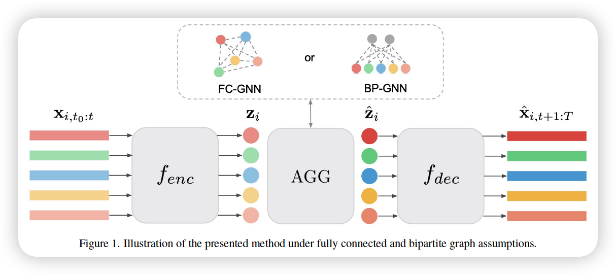
• Break down univariate model into 2 steps : \(f_{u}=f_{e n c} \circ f_{d e c}\)

  • \(\mathbf{x}_{i, t_{0}: t} \stackrel{f_{\text {enc }}}{\longrightarrow} \mathbf{z}_{i} \stackrel{f_{\text {dec }}}{\longrightarrow} \hat{\mathbf{x}}_{i, t+1: T}\).

• include a multivariate aggregation module \(A G G\) ,

  between \(f_{e n c}\) and \(f_{d e c}\)

  that propagate info among nodes in latent space \(\mathbf{z}=\left\{\mathbf{z}_{1}, \ldots, \mathbf{z}_{N}\right\}\)

  \(\rightarrow\) \(\hat{\mathbf{z}}=\mathrm{AGG}(\mathbf{z})\)

  ( this new embedding is passed to decoder )

\(\begin{aligned} \text { Univariate Encoder } & \mathbf{z}_{i}=f_{e n c}\left(\mathbf{x}_{i, t_{0}: t}, \mathbf{c}_{i}\right) \\ \text { Multivariate extension } & \hat{\mathbf{z}}=\mathrm{AGG}(\mathbf{z}) \\ \text { Univariate Decoder } & \hat{\mathbf{x}}_{i, t+1: T}=f_{d e c}\left(\hat{\mathbf{z}}_{i}\right) \end{aligned}\).

• overall model : multivariate
• but \(f_{e n c}\) and \(f_{d e c}\) : univariate

Does not propagate information among nodes at every time step,

but only in the AGG module \(\rightarrow\) CHEAPER!!!

(1) FC-GNN

• complexity : \(O(N^2)\)

• fully connected graph : \(\mathcal{G}=\{\mathcal{V}, \mathcal{E}\}\)

  • \(e_{i j}=1\) for all \(e_{i j} \in \mathcal{E}\)

• \(\mathbf{z}_{i}\) ( embedding of TS \(i\) ) is associated with \(v_{i} \in \mathcal{V}\)

  \(\rightarrow\) directly use GNN model as AGG

  \(\rightarrow\) the output node embedding \(\mathbf{h}_{i}^{L}\) is provided as the input \(\hat{\mathbf{z}}_{i}\) to decoder

• attention weights \(\alpha_{i j} \in(0,1)\) for each edge

  • “gate” the exchanged messages \(\mathbf{m}_{i}=\sum_{i \neq j} \alpha_{i j} \mathbf{m}_{i j}\)

    ( = dynamically inferring the graph )

    ( = just like \(\mathbf{m}_{i}=\sum_{j \in \mathcal{N}(i)} \mathbf{m}_{i j}=\sum_{j \neq j} e_{i j} \mathbf{m}_{i j}\) )

  • \(\sum_{i \neq j} e_{i j} \mathbf{m}_{i j} \approx \sum_{i \neq j} \alpha_{i j} \mathbf{m}_{i j}\) : can view it as

    • soft estimation \(\alpha_{i j}=\phi_{\alpha}\left(\mathbf{m}_{i j}\right)\)

(2) BP-GNN

• complexity : \(O(N K)\) …. \(K <<N\)
• bipartite graph : \(\mathcal{G}=(\mathcal{Y}, \mathcal{U}, \mathcal{E})\)
  • \(\mathcal{Y}\) : set of \(N\) nodes
    • associated embeddings : \(\mathbf{z}=\left\{\mathbf{z}_{1}, \ldots \mathbf{z}_{N}\right\}\)
  • \(\mathcal{U}\) : set of \(K\) auxiliary nodes
    • associated embeddings : \(\mathbf{u}=\left\{\mathbf{u}_{1}, \ldots \mathbf{u}_{K}\right\}\)
  • \(\mathcal{E}\) : edges, interconnecting all nodes between the two subsets \(\{\mathcal{Y}\), \(\mathcal{U}\}\)
    • but no connections among nodes within the same subset
    • total of \(2NK\) edges
• input to GNN : union of 2 node subsets \(\mathcal{V}=\mathcal{Y} \cup \mathcal{U}\)
  • input embedding : \(\mathbf{h}^{0}=\mathbf{z} \mid \mid \mathbf{u}\)
  • asynchronous schedule
    • (1) information is propagated from TS nodes to Auxiliary nodes ( \(\mathcal{Y} \rightarrow \mathcal{U}\) )
    • (2) vice versa ( \(\mathcal{U} \rightarrow \mathcal{Y}\) )

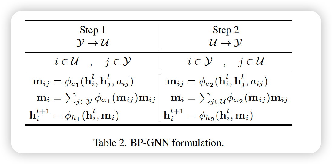
Define a adjacency matrices, correspoding to 2 message passing steps

• assuming all \(\alpha_{ij}=1\)

\(A_{1}= \mid \begin{array}{ll} 0_{N \times N} & 0_{N \times K} \\ 1_{K \times N} & 0_{K \times K} \end{array} \mid , \quad A_{2}= \mid \begin{array}{ll} 0_{N \times N} & 1_{N \times K} \\ 0_{K \times N} & 0_{K \times K} \end{array} \mid\).

• \(A_{1}\) refers to \(\mathcal{Y} \rightarrow \mathcal{U}\)
• \(A_{2}\) refers to \(\mathcal{U} \rightarrow \mathcal{Y}\)
• \(\tilde{A}=A_{2} A_{1}\) : sum of all paths that communicate the time series nodes \(\mathcal{Y}\) among each other through the auxiliary nodes \(\mathcal{U}\).