(paper) Structued Sequence Modeling with GCRN (2016)

Structued Sequence Modeling with GCRN (2016)

Contents

1. Abstract
2. Preliminaries
   1. Structured sequence modeling
   2. LSTM
   3. CNN on graphs
3. Proposed GCRN Models
   1. Model 1
   2. Model 2

0. Abstract

Introcues GCRN ( Graph Convolutional Recurrent Network )

• to predict structed sequences of data
• generalization of RNN to graph
• CNN + RNN
  • combines CNN on graphs for spatial structures
  • combines RNN on graph to find dynamic patterns

1. Preliminaries

(1) Structured sequence modeling

Sequence Modeling

= predicting the most likely future length \(k\) sequence, given past \(J\) observation

\(\rightarrow\) \(\hat{x}_{t+1}, \ldots, \hat{x}_{t+K}=\underset{x_{t+1}, \ldots, x_{t+K}}{\arg \max } P\left(x_{t+1}, \ldots, x_{t+K} \mid x_{t-J+1}, \ldots, x_{t}\right)\)

Example) n-gram LM ( with \(n= J+1\) )

• \(P\left(x_{t+1} \mid x_{t-J+1}, \ldots, x_{t}\right)\).

This paper

• special structued sequences, where \(x_t\) are NOT INDEPENDENT ( linked by pairwise relationship )
• \(x_{t}\) = graph signal

Notation :

• \(\mathcal{G}=(\mathcal{V}, \mathcal{E}, A)\), where \(\mid \mathcal{V} \mid =n\)

• \(A \in \mathbb{R}^{n \times n}\) : weighted adjacency matrix
• \(x_{t} \in \mathbb{R}^{n \times d_{x}}\).

(2) LSTM

• pass

(3) CNN on graphs

Spectral formulation for the convolution operator

\(y=g_{\theta} *_{\mathcal{G}} x=g_{\theta}(L) x=g_{\theta}\left(U \Lambda U^{T}\right) x=U g_{\theta}(\Lambda) U^{T} x \in \mathbb{R}^{n \times d_{x}}\).

( meaning : signal \(x\) is filtered by \(g_{\theta}\) with an element-wise multiplication of its graph Fourier transform \(U^{T} x\) with \(g_{\theta}\) )

• graph signal : \(x \in \mathbb{R}^{n \times d_{x}}\)
• filter ( non-parametric kernel ) : \(g_{\theta}(\Lambda)=\operatorname{diag}(\theta)\)
  • where \(\theta \in \mathbb{R}^{n}\) is a vector of Fourier coefficients
• \(U \in \mathbb{R}^{n \times n}\) : matrix of eigen vectors
• \(\Lambda \in \mathbb{R}^{n \times n}\) : diagonal matrix of eigenvalues of the \(L\)
• \(L=I_{n}-D^{-1 / 2} A D^{-1 / 2}=U \Lambda U^{T} \in \mathbb{R}^{n \times n}\).

\(\rightarrow\) evaluating above : \(O(n^2)\)

Truncation up to \(K-1\) ( ChebNet )

Idea : parameterize \(g_{\theta}\) as a TRUNCATED expansion

• up to order \(K-1\) of Chebyshev polynomials \(T_{k}\)
• \(g_{\theta}(\Lambda)=\sum_{k=0}^{K-1} \theta_{k} T_{k}(\tilde{\Lambda})\).
  • (1) \(\theta \in \mathbb{R}^{K}\) is a vector of Chebyshev coefficients
  • (2) \(T_{k}(\tilde{\Lambda}) \in \mathbb{R}^{n \times n}\) is the Chebyshev polynomial of order \(k\), where \(\tilde{\Lambda}=2 \Lambda / \lambda_{\max }-I_{n}\)

Graph Filtering Operation :

\(y=g_{\theta} *_{\mathcal{G}} x=g_{\theta}(L) x=\sum_{k=0}^{K-1} \theta_{k} T_{k}(\tilde{L}) x\).

• where \(T_{k}(\tilde{L}) \in \mathbb{R}^{n \times n}\) is the Chebyshev polynomial of order \(k\) ,

  evaluated at scaled Laplacian \(\tilde{L}=2 L / \lambda_{\max }-I_{n}\)

\(\rightarrow\) complexity reduction : \(\mathcal{O}(K \mid \mathcal{E} \mid )\) … linearly with the number of edges

\(\rightarrow\) meaining : \(K\)-neighborhood

2. Proposed GCRN Models

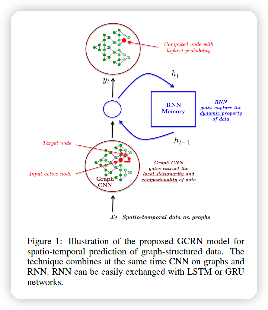
propose 2 GCRN architectures.

(1) Model 1

Idea = stack a graph CNN & LSTM

\(\begin{aligned} x_{t}^{\mathrm{CNN}} &=\mathrm{CNN}_{\mathcal{G}}\left(x_{t}\right) \\ i &=\sigma\left(W_{x i} x_{t}^{\mathrm{CNN}}+W_{h i} h_{t-1}+w_{c i} \odot c_{t-1}+b_{i}\right), \\ f &=\sigma\left(W_{x f} x_{t}^{\mathrm{CNN}}+W_{h f} h_{t-1}+w_{c f} \odot c_{t-1}+b_{f}\right), \\ c_{t} &=f_{t} \odot c_{t-1}+i_{t} \odot \tanh \left(W_{x c} x_{t}^{\mathrm{CNN}}+W_{h c} h_{t-1}+b_{c}\right), \\ o &=\sigma\left(W_{x o} x_{t}^{\mathrm{CNN}}+W_{h o} h_{t-1}+w_{c o} \odot c_{t}+b_{o}\right), \\ h_{t} &=o \odot \tanh \left(c_{t}\right) . \end{aligned}\).

(2) Model 2

Idea = replace CNN to GCN in Model 1

\(\begin{aligned} i &=\sigma\left(W_{x i} *_{\mathcal{G}} x_{t}+W_{h i} *_{\mathcal{G}} h_{t-1}+w_{c i} \odot c_{t-1}+b_{i}\right), \\ f &=\sigma\left(W_{x f} *_{\mathcal{G}} x_{t}+W_{h f} *_{\mathcal{G}} h_{t-1}+w_{c f} \odot c_{t-1}+b_{f}\right), \\ c_{t} &=f_{t} \odot c_{t-1}+i_{t} \odot \tanh \left(W_{x c} *_{\mathcal{G}} x_{t}+W_{h c} *_{\mathcal{G}} h_{t-1}+b_{c}\right), \\ o &=\sigma\left(W_{x o} *_{\mathcal{G}} x_{t}+W_{h o} *_{\mathcal{G}} h_{t-1}+w_{c o} \odot c_{t}+b_{o}\right), \\ h_{t} &=o \odot \tanh \left(c_{t}\right) . \end{aligned}\).