(paper) MTHetGNN ; A Heterogeneous Graph Embedding Framework for MTS forecasting

MTHetGNN : A Heterogeneous Graph Embedding Framework for MTS forecasting (2020)

Contents

1. Abstract
2. Introduction
3. Previous Works
   1. Heterogeneous Network Embedding
4. Framework
   1. Task Formulation
   2. Model Architecture
   3. Temporal Embedding Module
   4. Relation Embedding Module
   5. Heterogeneous Graph Embedding Module
5. Objective Function

0. Abstract

modeling complex relations

• not only essential in characterzing latent dependency & modeling temporal dependence
• but also brings great challenges in MTS forecasting task

Existing methods

• mainly focus on modeling certain relations among MTS variables

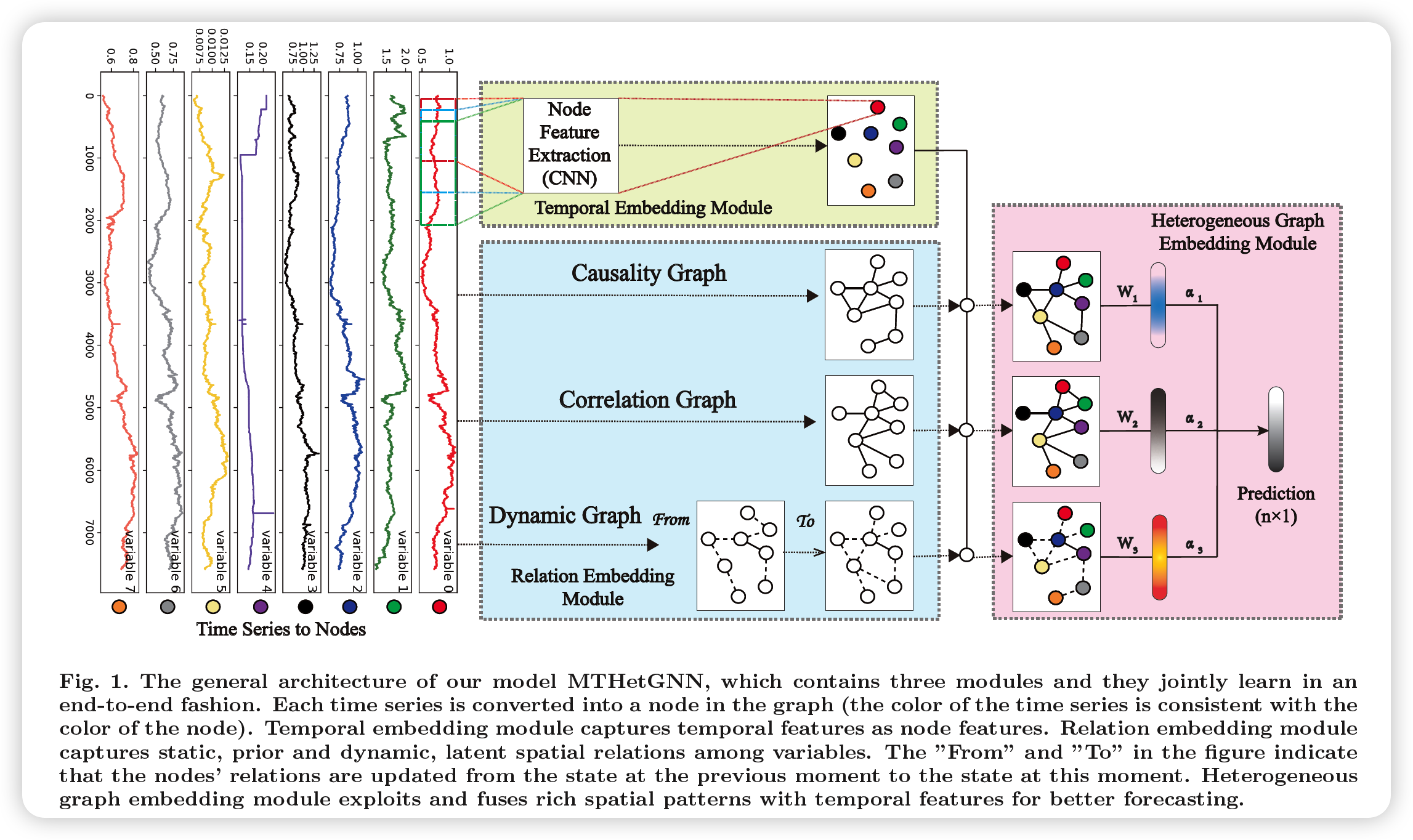
MTHetGNN

• novel end-tn-end DL model

• (1) RELATION EMBEDDING module

  • to characterize complex relations among variables
  • structure
    • each variable = node
    • specific static/dynamic relationships = edge

• (2) TEMPORAL EMBEDDING module

  • for TS feature extraction
  • CNN filters, with different perception scales

• (3) HETEROGENEOUS GRAPH EMBEDDING module

  • Adopted to handle the complex structural information,

    generated by the above 2 modules

1. Introduction

core of MTS forecasting … 2 significant characteristics

• (1) the internal temporal dependenc of each TS

  • ex) sun spot of time \(T\) & \(T+k\) may be correlated
• (2) the rich spatial relations among different TSs
  • ex) traffic forecasting

• there also ecsists relations among variables,

  that are unknown/ changing over time

Limitation in exploiting latent and rich interdependencies among variables efficiently and effectively!!

Previous algorithms

• ARIMA / VAR / AR : skip
• LSTNet / MLCNN :
  • consider long-term dependency & short-term variance for TS
  • but cannot explicitly model the pairwise dependencies among TSs
• MTS with GNN
  • TEGNN / MTGNN :
    • can only reveal one type of relation
    • lack the ability to model both static & dynamic relations in TS

MTHetGNN summary

• embed each relation/interdependency into graph structure

• fuses all graph structures & temporal features

• 3 modules

  • Relation embedding module
    • considers (1) static/prior & (2) dynamic/latent relations among variables
      • (1) static/prior : global relations
      • (2) dynamic/latent : dynamic local relations
  • Temporal embedding module
    • CNN for TS feature extractuin
  • Heterogeneous graph embedding module
    • input : output of 2 modules above
    • tackle the complex structural embedding of graph structure

Contribution

• propose a HETEROGENEOUS GNN for MTS
• construcxt relation embedding module to explore the “relations among TS” in both DYNAMIC & STATIC approaches

2. Previous Works

(1) Heterogeneous Network Embedding

start with extraction of typed structural features

• problem?
  • need to consider structural info, composed of multiple types of nodes & edges
  • many methods dealing with heterogeneous networks involve META STRUCTURE
• Ex) metapath2vec
  • uses path composed of nodes, obtained from RW, guided by metapath
• Ex) NSHE

Attention mechanism to Heterogeneous graphs

• HAN : uses metapath to model higher-order similarities & uses attention
• HGAT : use a dual-level attention
  • (1) nodel-level attention
    • importance of nodes & neighbors, based on meta-paths
  • (2) type-level attention
    • importance of different meta-paths
  • fully consider the rich information in heterogeneous graphs
• SR-HGAT
  • considers characterisitics of nodes & high-order relations simultaneously
  • uses an aggregator based on 2 layer attention, to capture basic semantics effectively
• RAM ( GAT with a Relation Attention Moudle )

3. Framework

(1) Task Formulation

MTS : \(X_{i}=\left\{x_{i 1}, x_{i 2}, \ldots, x_{i T}\right\}\)

• \(x_{i t} \in \mathcal{R}^{n}\) : \(n\) 개의 variable, at time \(t\), from \(i^{th}\) sample
• (참고) 1개의 time series 내에도, 여러 개의 변수가 존재할 수 있다!

Task : predict the future value \(x_{t+h}\)

• input : \(\mathcal{X}=\left\{X_{1}, X_{2}, \ldots, X_{s}\right\}\)
• output : \(\mathcal{Y}=\left\{Y_{1}, Y_{2}, \ldots, Y_{s}\right\}\)

(2) Model Architecture

(3) Temporal Embedding Module

GOAL : capture temporal features by multiple CNN

• different receptive fields ( like inception module )

  ( use \(p\) CNN filters, with kernel size \(1 \times k_i\) )

• ex) [1x3, 1x5, 1x7]

(4) Relation Embedding Module

GOAL : learn graph adjacency matrix

• model implicit relations in MTS variables
• both static & dynamic strategies

Static perspective

• use (1) correlation coefficient & (2) transfer entropy

  to model static linear relationships and implicit causality among variables

Dynamic perspective

• adopt (3) dyanamic graph learning & learn graph structure adaptively
• modeling time-varying graph structure

Summary : varies adjacency matrices are generated and then fed into heterogeneous GNN to interpret the relations between graph nodes in both static and dynamic way

Notation

• MTS : \(\mathcal{X}=\left\{X_{1}, X_{2}, \ldots, X_{s}\right\}\)

• (1) similarity adjacency matrix : \(A^{\operatorname{sim}} \in \mathcal{R}^{n \times n}\)

  • \(A^{\operatorname{sim}}=\operatorname{Similarity}(\mathcal{X})\).

  • measure pairwise similarity between TSs

• (2) causality adjacency matrix : \(A^{\text {cas }} \in \mathcal{R}^{n \times n}\)

  • \(A^{\text {cas }}=\text { Causality }(\mathcal{X})\).
  • measure causality between TSs

• (3) adaptive adjacency matrix : \(A^{D A} \in \mathcal{R}^{n \times n}\)

  • \(A^{d y}=\text { Evolve }\left(X_{i}\right)\).

a) Similarity Adjacency matrix

to measure the global correlation among TSs

metric ex)

• Euclidean distance
• Landmark similarity

• DTW

• correlation & coefficient (v)

\(A_{i j}^{s i m}=\frac{\operatorname{Cov}\left(X_{i}, X_{j}\right)}{\sqrt{D\left(X_{i}\right)} \sqrt{D\left(X_{j}\right)}}\).

• \(D\left(X_{i}\right)\) : variance of TS \(X_i\)

b) Causality Adjacency matrix

metric ex)

• Granger Causality
• Transfer Entropy (v)

Transfer Entropy (TE)

• use TE to process non-stationary TS
• pseudo-regression relationship will b e produced
• (formula) TE of variable \(A\) to \(B\) :
  • \(T_{B \rightarrow A}=H\left(A_{t+1} \mid A_{t}\right)-H\left(A_{t+1} \mid A_{t}, B_{t}\right)\).

Notation

• \(m_t^{(k)}\) : \(\left[m_{t}, m_{t-1}, \ldots, m_{t-k+1}\right]\)
  • \(m_{t}\) : value of variable \(m\) at time \(t\)
  • \(k\) : window size
• \(H\left(M_{t+1} \mid M_{t}\right)\) : conditional entropy
  • \(H\left(M_{t+1} \mid M_{t}\right)=\sum p\left(m_{t+1}, m_{t}^{(k)}\right) \log _{2} p\left(m_{t+1} \mid m_{t}^{(k)}\right)\).
• using conditional entropy, we can get \(A^{\text {cas }}\)
  • \(A_{i j}^{c a s}=T_{X_{i} \rightarrow X_{j}}-T_{X_{j} \rightarrow X_{i}}\).

c) adaptive adjacency matrix

( = dynamic evolving network )

learns the adjacency matrix adaptively!!

\(A^{d y}=\text { Evolve }\left(X_{i}\right)\),

( \(A^{d y}=\sigma(D W)\) )

• \(D_{i j}=\frac{\exp \left(-\sigma\left(\text { distance }\left(x_{i}, x_{j}\right)\right)\right)}{\sum_{p=0}^{n} \sigma\left(\exp \left(-\sigma\left(\text { distance }\left(x_{i}, x_{p}\right)\right)\right)\right.}\).
  • where \(x_{i}, x_{j}\) denote the \(i^{t h}, j^{t h}\) time series
  • input TS : \(X_{k}=x_{1}, x_{2}, \ldots, x_{n} \in \mathcal{R}^{n \times T}\)
    • \(n\) : number of time series
    • \(T\) : number of time length
    • \(k\) : \(k^{th}\) sample ( = \(k^{th}\) graph )

Other techniques

Normalization

• Normalization is applied to the output of each strategy respectively to form three normalized adjacency matrix

Threshold

• \(A_{i j}^{r}=\left\{\begin{array}{rc} A_{i j}^{r} & A_{i j}^{r}>=\text { threshold } \\ 0 & A_{i j}^{r}<\text { threshold } \end{array}\right.\).

(5) Heterogeneous Graph Embedding Module

Can be viewed as a graph based aggregation method

• fuses (1) temporal features & (2) spatial relations between TS

motivated by R-GCNs

• learns an aggregation function that is representation-invariant
• can operate on large-scale relational data

Attention Mechanism

Fuse node embeddings of each heterogeneous graph with attention mechanism

• \(H^{(l+1)}=\sigma\left(H^{(l)} W_{0}^{l}+\sum_{r \in \mathcal{R}} \operatorname{softmax}\left(\alpha_{r}\right) \hat{A}_{r} H^{(l)} W_{r}^{(l)}\right)\).
  • \(H^{(0)}=X\).
  • \(\alpha_{(r)}\) : weight coefficient of each heterogeneous graph
  • \(\operatorname{softmax}\left(\alpha_{r}\right)=\frac{\exp \left(\alpha_{r}\right)}{\sum_{i=1}^{ \mid R \mid } \exp \left(\alpha_{i}\right)} \cdot W_{o}^{(l)}\).

4. Objective Function

\(L_2\) loss is widely used.

\(\operatorname{minimize}\left(\mathcal{L}_{2}\right)=\frac{1}{k} \sum_{i}^{k} \sum_{j}^{n}\left(y_{i j}-\hat{y}_{i j}\right)^{2}\).

\(L_1\) loss has a stable gradient for different inputs

( reduce impact of outliers & avoid gradient explosions )

\(\operatorname{minimize}\left(\mathcal{L}_{1}\right)=\frac{1}{k} \sum_{i}^{k} \sum_{j}^{n} \mid y_{i j}-\hat{y}_{i j} \mid\).