(paper) Predicting Path Failure in Time-Evolving Graphs

Predicting Path Failure in Time-Evolving Graphs (2019)

Contents

1. Abstract
2. Problem Definition
3. Methodology
   1. Framework
   2. Time-Evolving Graph Modeling

0. Abstract

Time-evolving graph

• sequence of graph snapshots (\(G_1, \cdots G_t\) )
• used to solve path classification

to capture temporal dependency & graph structure dynamics

\(\rightarrow\) design a novel DNN named LRGCN ( = LSTM R-GCN )

LRGCN

• considers temporal dependency between time-adjacenct graph snapshots,

  as a spetial relation with memory

• use R-GCN to jointly process (1) intra & (2) inter time relations

• Propose “new path representation method”, named SAPE

  ( SAPE = Self-Attentive Path Embedding )

  \(\rightarrow\) embed paths of arbitrary length, into fixed-length vectors

1. Problem Definition

Notation of Time Evolving Graph

• nodes : \(V=\left\{v_{1}, v_{2}, \ldots, v_{N}\right\}\)
• \(\boldsymbol{A}=\left\{A^{0}, A^{1}, \ldots, A^{t}\right\}\);
  • \(A^t\) : \(N\times N\) adjacency matrix at time \(t\)
• \(\boldsymbol{X}=\left\{X^{0}, X^{1}, \ldots, X^{t}\right\}\).
  • \(X^{t}=\left\{x_{1}^{t}, x_{2}^{t}, \ldots, x_{N}^{t}\right\}\) : observation of each node, at time \(t\)
    • \(x_{i}^{t} \in \mathbb{R}^{d}\) ( ex. temperature, power, signals … )
• Path : sequence \(p=\left\langle v_{1}, v_{2}, \ldots, v_{m}\right\rangle\) of length \(m\)
• observations of the path nodes at time \(t\) : \(s^{t}=\left\langle x_{1}^{t}, x_{2}^{t}, \ldots, x_{m}^{t}\right\rangle\)

( focus on Directed graph )

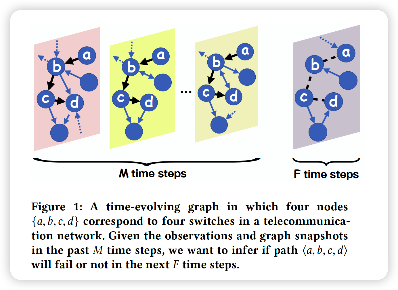
Goal : predict if a given path is available or not in the future

• For a given path \(p\) at time \(t\),

  use past \(M\) time steps

  to predict the availability of this path in the next \(F\) time steps.\

• formulate it as classification problem

• ex) path failure in telecommunication network

Loss Function :

\(\arg \min \mathcal{L}=-\sum_{\boldsymbol{P}_{j} \in D} \sum_{c=1}^{C} Y_{j c} \log f_{c}\left(\boldsymbol{P}_{j}\right)\).

• train data : \(\boldsymbol{P}_{j}=\left(\left[s_{j}^{t-M+1}, \ldots, s_{j}^{t}\right], p_{j},\left[A^{t-M+1}, \ldots, A^{t}\right]\right)\).
• train label : \(Y_{j} \in\{0,1\}^{C}\) …….. availability of this path

2. Methodology

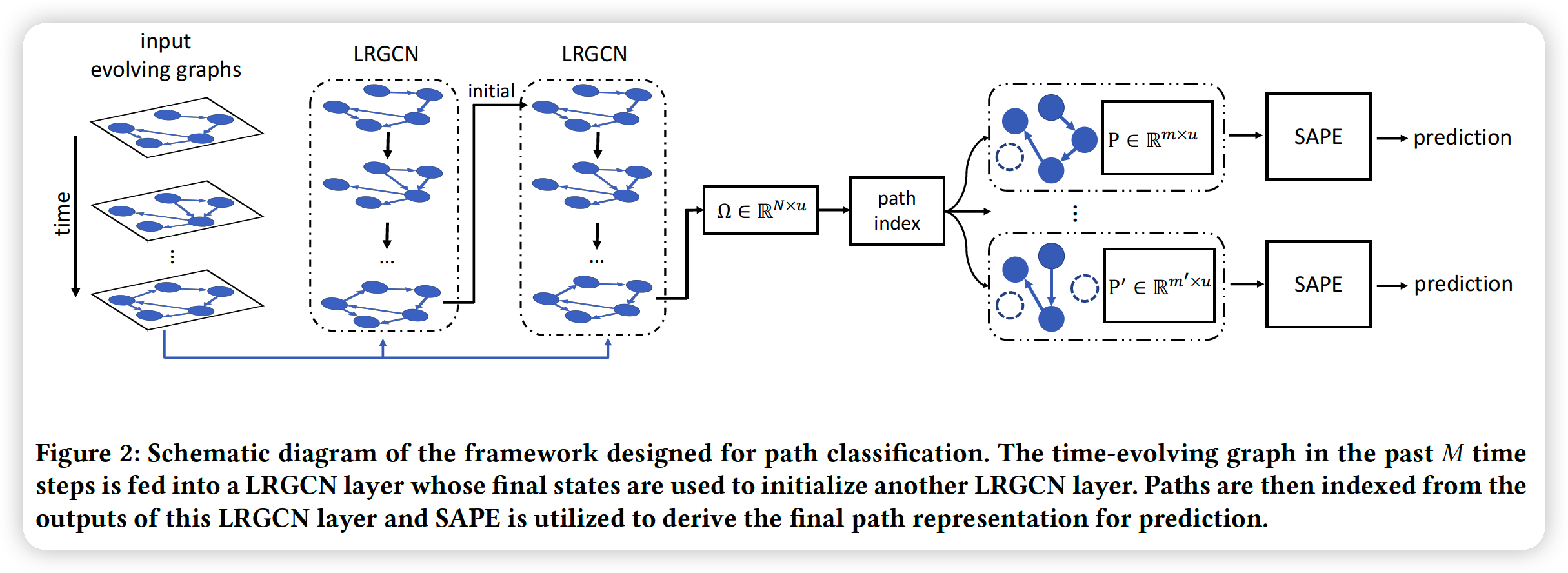
(1) Framework

3 important properties in time-evolving graph

1. node correlation
2. influence of graph structure dynamics
   • node features are influenced by change of graph structure
3. temporal dependency

(2) Time-Evolving Graph Modeling

new time-evolving NN

• to capture “graph structure dynamics” & “temporal dependency” jointly

• GCN : can not take both \(X\) and evolving structures \(A\) as input

  \(\rightarrow\) LRGCN focus on “how to generalize GCN to process TS & evolving graph structures simultaneoulsy”

a) Static Graph modeling

WITHIN on graph snapshot

• structure does not change = “static”

• GCN & R-GCN

  • original GCN : deals with “static” graph

  • R-GCN : deal with “multi-relational graph”

    • ex) directed graph

This paper

• use R-GCN to model the node correlation in “static & directed graph”

• R-GCN ( ex. for “directed graph” )
  • \(Z=\sigma\left(\sum_{\phi \in R}\left(D_{\phi}^{t}\right)^{-1} A_{\phi}^{t} X^{t} W_{\phi}+X^{t} W_{0}\right)\).
    • where \(R=\{\) in, out }
    • \(A_{i n}^{t}=A^{t}\) & \(A_{o u t}^{t}=\left(A^{t}\right)^{T}\)
  • \(\left(D_{\phi}^{t}\right)_{i i}= \sum_{j}\left(A_{\phi}^{t}\right)_{i j} . \sigma(\cdot)\).
• Generalization of R-GCN
  • \(Z_{s}=\sigma\left(\sum_{\phi \in R} \tilde{A}_{\phi}^{t} X^{t} W_{\phi}\right)\).
    • \[\tilde{A}_{\phi}^{t}=\left(\hat{D}_{\phi}^{t}\right)^{-1} \hat{A}_{\phi}^{t}\]
    • \[\hat{A}_{\phi}^{t}=A_{\phi}^{t}+I_{N}\]
    • \[\left(\hat{D}_{\phi}^{t}\right)_{i i}=\sum_{j}\left(\hat{A}_{\phi}^{t}\right)_{i j}\]
• can impose multi-hop normalization by stacking multiple R-GCN
  • ex) 2 layer R-GCN : \(\Theta_{s} \star g X^{t}=\sum_{\phi \in R} \tilde{A}_{\phi}^{t} \sigma\left(\sum_{\phi \in R} \tilde{A}_{\phi}^{t} X^{t} W_{\phi}^{(0)}\right) W_{\phi}^{(1)}\)

LR-GCN

• Extend R-GCN to take as inputs 2 adjacent graph snapshots

b) Adjacent Graph Snapshots modeling

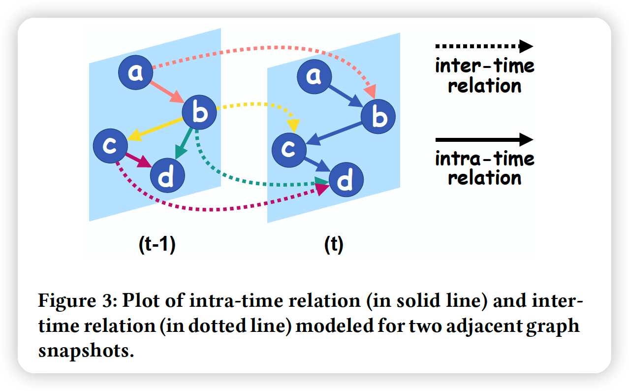
• 2 adjacent time steps ( \(t-1\) & \(t\) )

INTER-time relation

• relationship with nodes in time \(t-1\)

INTRA-time relation

• relationship with nodes in time \(t\)

( both are “asymmetric & directed” relations )

4 types of relations to model in R-GCN

• (1) intra-incoming
• (2) intra-outgoing
• (3) inter-incoming
• (4) inter-outgoing

\(G_{-} \text {unit }\left(\Theta,\left[X^{t}, X^{t-1}\right]\right)=\sigma\left(\Theta_{S} \star g X^{t}+\Theta_{h} \star g X^{t-1}\right)\).

• \(\Theta_{h}\) : parameters for “inter-time” modeling

  ( does not change over time )

• similar role as RNN

c) LRGCN

• use a \(H^{t-1}\) to memorize the transformed features in the previous snapshots

• feed \(H^{t-1}\) & \(X^{t}\) into the unit & get \(H^t\)

  • \(H^{t}=\sigma\left(\Theta_{H} \star g\left[X^{t}, H^{t-1}\right]\right)\).

• still problem …… gradient exploding/vanishing

  \(\rightarrow\) use LSTM … that is LR-GCN