(paper) Multi-scale temporal feature extraction based GCN with Attention for MTS Prediction

Multi-scale temporal feature extraction based GCN with Attention for MTS Prediction (2022)

Contents

1. Abstract

2. Introduction

   1. EMD
   2. GCN

3. Related Works

4. Preliminaries

   1. EMD
   2. TCN

5. Proposed Approach

   1. Feature Extraction of TS by EMD
   2. Graph Generation
   3. Node Feature updating

   4. Establishment of Temporal relationships

   5. Loss Function

0. Abstract

Overview

• propose a novel GNN, based on MULTI_scale temporal feature extraction

• use attention mechanism

3 key points

(1) Empirical Modal Decomposition (EMD)

• to extract time-domain features

(2) GCN

• to generate node embeddings that contain spatial relationships

(3) TCN

• to capture temporal relationships for the node embedding

1. Introduction

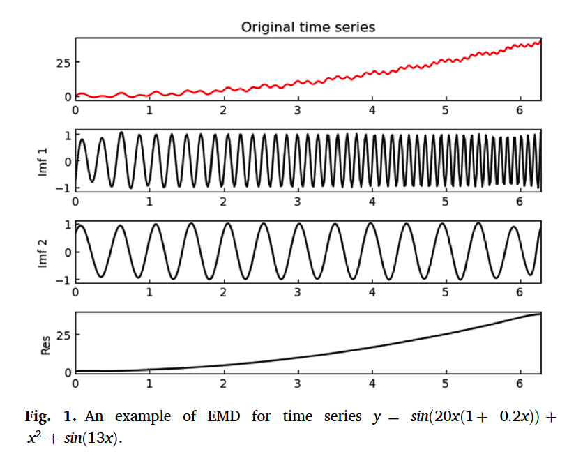
(1) EMD ( Empirical Mode Decomposition )

• signal processing tehcnique
• to deal with unstable & non-linear sequences
• used to “extract TEMPORAL FEATURES at DIFFERENT TIME SCALES”

(2) GCN

• used for node feature updating
• and generating node embeddings

2. Related Works

( check GConvLSTM & GConvGRU )

appropriate temporal feature extraction methods are crucial!!

3. Preliminaries

(1) EMD ( Empirical Mode Decomposition )

Decompose TS into several different intrinsic mode functions (IMFs) & residuals

\(\boldsymbol{x}=\sum_{i=1}^{N} \boldsymbol{i m} \boldsymbol{f}_{i}+\boldsymbol{r}_{N}4\).

• \(\boldsymbol{i m f}_{i}\) : the \(i\) th IMF
• \(N\) : number of IMFs.

(2) TCN

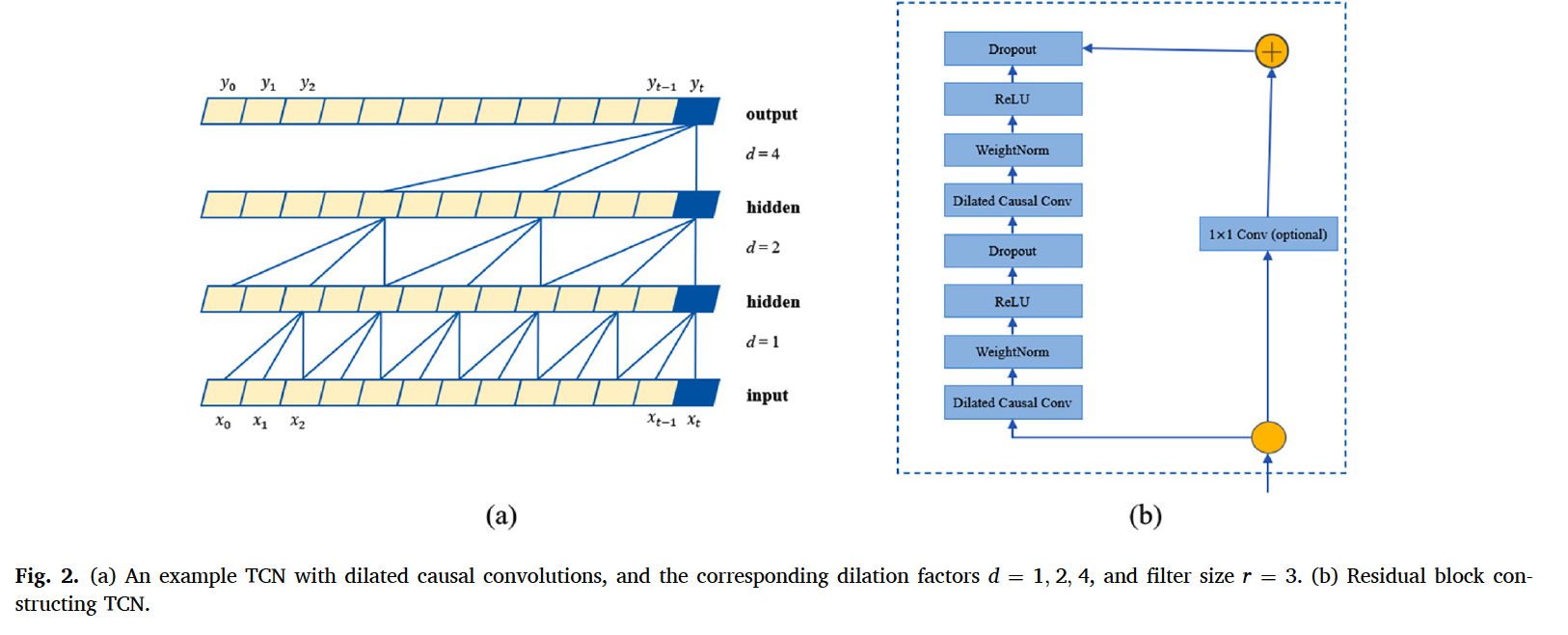
• able to capture long-term dependencies
• use residual blocks

4. Proposed Approach

consists of 4 parts

1. Feature Extraction
2. Graph Generation
3. Node Feature Updating
4. Establishment of Temporal Relationship

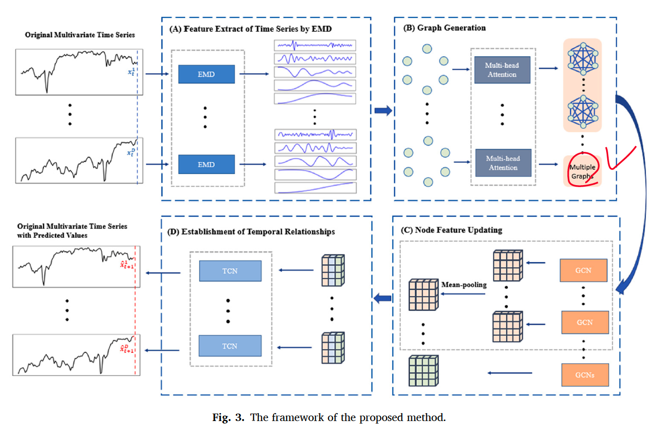
(1) Feature Extraction of TS by EMD

Original TS : noisy & outliers

use EMD to decompose original TS

• meaning of each component : different time scale features
• can mitigate effect of noise

MTS : \(\boldsymbol{X}=\left\{\boldsymbol{x}_{1}, \boldsymbol{x}_{2}, \ldots, \boldsymbol{x}_{T}\right\}\).

• where \(\boldsymbol{x}_{t} \in \mathbb{R}^{D}\)
• \(j^{th}\) dimensional TS : \(\boldsymbol{X}^{j}=\{\left.x_{1}^{j}, x_{2}^{j}, \ldots, x_{T}^{j}\right\}\)

Decomposition of \(\boldsymbol{X}^{j}\)

• \(\boldsymbol{X}^{j}=\sum_{i=1}^{N} \boldsymbol{i m f}_{i}^{j}+\boldsymbol{r}_{N}^{j}\).

Matrix Notation

\(\boldsymbol{M}^{j}=\left[\begin{array}{cccc} i m f_{1}^{j}(1) & i m f_{1}^{j}(2) & \cdots & i m f_{1}^{j}(T) \\ i m f_{2}^{j}(1) & i m f_{2}^{j}(2) & \cdots & i m f_{2}^{j}(T) \\ \vdots & \vdots & \ddots & \vdots \\ i m f_{N}^{j}(1) & \operatorname{imf}_{N}^{j}(2) & \cdots & i m f_{N}^{j}(T) \\ r_{N}^{j}(1) & r_{N}^{j}(2) & \cdots & r_{N}^{j}(T) \end{array}\right]\).

• each subsequence obtained by EMD : used as node features

(2) Graph Generation

each subsequence obtained by EMD

= different time scale features of original TS

\(\rightarrow\) used to characterize nodes

Sliding window ( size \(k\) )

• divide each dimensional feature matrix
• obtain \(\boldsymbol{M}^{1}[T-k+1: T]\) ….\(\boldsymbol{M}^{D}[T-k+1: T]\)

Concatenate “IMFs” & “residuals”

\(\boldsymbol{V}_{t}=\left[\boldsymbol{v}_{t}^{1}, \boldsymbol{v}_{t}^{2}, \ldots, \boldsymbol{v}_{t}^{D}\right]^{T}=\left[\begin{array}{ccccc} \operatorname{imf}_{1}^{1}(T-t+1) & \operatorname{imf}_{2}^{1}(T-t+1) & \cdots & \operatorname{imf}_{N}^{1}(T-t+1) & r_{N}^{1}(T-t+1) \\ \operatorname{imf}_{1}^{2}(T-t+1) & \operatorname{imf}_{2}^{2}(T-t+1) & \cdots & \operatorname{imf}_{N}^{2}(T-t+1) & r_{N}^{2}(T-t+1) \\ \vdots & \vdots & \ddots & \vdots & \vdots \\ \operatorname{imf}_{1}^{D}(T-t+1) & \operatorname{imf}_{2}^{D}(T-t+1) & \cdots & \operatorname{imf}_{N}^{D}(T-t+1) & r_{N}^{D}(T-t+1) \end{array}\right]\).

• \(V_{t} \in \mathbb{R}^{D \times(N+1)}\) : initial node feature matrix at \(t\) moment
  • \(v_{t}^{j} \in \mathbb{R}^{N+1}\) : initial feature vector of the \(j\) th node of the graph at \(t\) moment.

Multi-head attention

\(\tilde{\boldsymbol{A}}^{i}=\operatorname{softmax}\left(\frac{\boldsymbol{Q} \boldsymbol{W}_{i}^{Q} \times\left(\boldsymbol{K} \boldsymbol{W}_{i}^{K}\right)^{T}}{\sqrt{N+1}}\right)\).

• \(\boldsymbol{Q} \in \mathbb{R}^{D \times(N+1)}\) & \(\boldsymbol{K} \in \mathbb{R}^{D \times(N+1)}\) : node feature matrix

  • \(N+1\) : dimension of node features

• \(\tilde{\boldsymbol{A}}^{i}\) : \(i\)th adjacency matrix

  • \(i \in\{1, 2, \ldots, \alpha\}\). ( number of heads )

  • When the prior knowledge of MTS ….

    \(\widetilde{\boldsymbol{A}}^{i}=\operatorname{softmax}\left(\frac{\boldsymbol{Q} \boldsymbol{W}_{i}^{Q} \times\left(\boldsymbol{K} \boldsymbol{W}_{i}^{K}\right)^{T}}{\sqrt{N+1}}\right) \boldsymbol{A}\).

Learnt adjacency matrix

• varies with input!

• multiple matrices, with multi-head attention

  ( \(\alpha\) FC graphs for all \(k\) moments )

(3) Node feature updating

• use GCN to generate embeddings of nodes

• for \(i^{th}\) graph at a given moment..

  • \(\boldsymbol{H}_{i}^{l+1}=\rho\left(\widetilde{\boldsymbol{A}}^{i} \boldsymbol{H}_{i}^{l} \boldsymbol{W}_{i}^{l+1}+\boldsymbol{b}_{i}^{l+1}\right)\).
    • \(\boldsymbol{H}_{i}^{l} \in \mathbb{R}^{D \times h_{\text {din }}}, l=\{1,2, \ldots, J\}\) : hidden matrix
    • \(\boldsymbol{H}_{i}^{0}\) : initial node feature matrix

Embedding for the \(t\) moment :

• \(\boldsymbol{E}_{t}=\) MeanPooling \(\left(\boldsymbol{H}_{i}^{J}, \alpha\right)\)
  • \(\boldsymbol{E}_{t}=\left[\boldsymbol{e}_{t}^{1}, \boldsymbol{e}_{t}^{2}, \ldots, \boldsymbol{e}_{t}^{D}\right]^{T}, t=\{1,2, \ldots, k\}\),
  • \(\boldsymbol{e}_{t}^{j} \in \mathbb{R}^{h_{\text {ouput }}}\) : \(j\) th node embedding at the \(t\) moment

(4) Establishment of temporal relationships

Input : \(\boldsymbol{E}^{j}=\left[\boldsymbol{e}_{1}^{j}, \boldsymbol{e}_{2}^{j}, \ldots, \boldsymbol{e}_{k}^{j}\right]\)

use TCN

(5) Loss Function

\(\operatorname{loss}=\frac{1}{D(T-1)} \sum_{j=1}^{D} \sum_{t=1}^{T}\left(x_{t}^{j}-\widehat{x}_{t}^{j}\right)^{2}\).

• GCN & TCN are jointly learned