
Neural Additive Models : Interpretable Machine Learning with Neural Nets
Contents
- Abstract
- Introduction
- NAMs (Neural Additive Models)
- Fitting Jagged Shape Functions
- Regularization & Training
- Intelligibility & Modularity
0. Abstract
DNNS = BLACK-BOX model ( unclear how they make decisions )
이 논문은 NAMs (Neural Additive Models)를 제안한다
NAM은 아래의 두 가지 (1) + (2)의 특징을 결합한다
- (1) expressitivity of DNNs
- (2) Inherent intelligibility of GAM (Generalized Additive Models)
요약 : NAM은 각각의 input feature에 대한 NN 들의 linear combination을 학습한다!
1. Introduction
NAMs는 더 큰 family인 GAM (Generalized Additive Models)에 속한다!
GAM의 형태 :
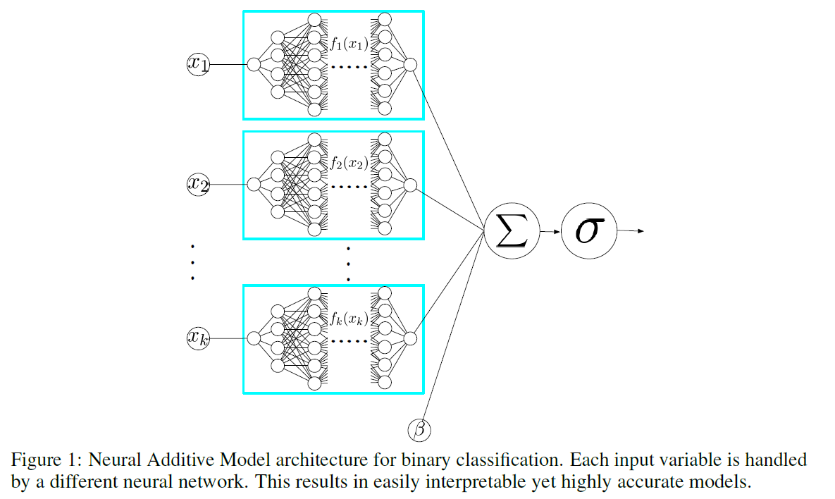
- \(g(\mathbb{E}[y])=\beta+f_{1}\left(x_{1}\right)+f_{2}\left(x_{2}\right)+\cdots+f_{K}\left(x_{K}\right)\).
- \(\mathrm{x}=\left(x_{1}, x_{2}, \ldots, x_{K}\right)\) : \(K\) features의 input
- \(g(.)\) : link function ( ex. logistic function )
- \(f_{i}\) is a univariate shape function with \(\mathbb{E}\left[f_{i}\right]=0\)
NAMs : linear combination of networks를 학습한다
-
하나의 network는 하나의 input feature에 대해 모델링
-
trained jointly using back-prop
-
NAMs에 대한 해석은 매우 쉽다!
( \(\because\) impact of a feature on prediction does not rely on other features )
NAM의 advantages
- expressive & intelligible
- likely to combine with other DL methods
- due to flexibility of NNs, can be easily extended to various settings problematic for boosted decision trees
- can be trained on GPUs
2. NAMs (Neural Additive Models)
2-1) Fitting Jagged Shape Functions
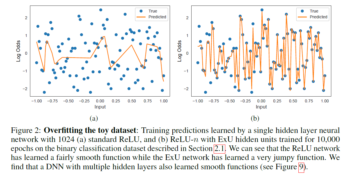
Jagged function을 모델링하는 것은 중요하다!
( 현실에는 sharp jump들이 많다! ( 그림으로 이해) )
-
“GAMS fit using spline” = OVER regularize! ( \(\rightarrow\) 낮은 성능 )
-
따라서, NN을 사용하여 non-linear shape function을 학습하자!
- 하지만, standard NNs fail to model highly jumpy 1D functions
\(\rightarrow\) 이 논문은, exp-centered (ExU) hidden units를 제안한다!
ExU : \(h(x)=f\left(e^{w} *(x-b)\right)\)
- 위에서 말한 NN이 highly jumpy function 포착 못하는 단점을 극복하기 위해!
-
learn \(w\) & \(b\)
-
ExU의 intuition
-
hidden unit은 ( 작은 input의 변화로도 ) output을 급격히 바꿀 수 있어야 한다
-
sharpness에 따라 \(w\)가 다르게 학습된다
-
- 제안하는 initial weight : \(N(x,0.5)\), with \(x \in [3,4]\)
2-2) Regularization & Training
- Dropout
- Weight Decay
- Output Penalty ( L2 norm 사용 )
- Feature Dropout
- dropout individual feature networks
Training
Notation
- training data : \(\mathcal{D}=\left\{\left(\mathbf{x}^{(i)}, y^{(i)}\right)\right\}_{i=1}^{N}\)
- \(\mathrm{x}=\) \(\left(x_{1}, x_{2}, \ldots, x_{K}\right)\) contains \(K\) features
- Loss Function : \(\mathcal{L}(\theta)\)
Loss Function
\(\mathcal{L}(\theta)=\mathbb{E}_{x, y \sim \mathcal{D}}\left[l(x, y ; \theta)+\lambda_{1} \eta(x ; \theta)\right]+\lambda_{2} \gamma(\theta)\).
- \(\eta(x ; \theta)=\frac{1}{K} \sum_{x} \sum_{k}\left(f_{k}^{\theta}\left(x_{k}\right)\right)^{2}\) : output penalty
- \(\gamma(\theta)\) : weight decay
- feature dropout and dropout with coefficients \(\lambda_{3}\) and \(\lambda_{4}\)
Regression의 경우
- \(l(x, y ; \theta)=-y \log \left(p_{\theta}(x)\right)-(1-y) \log \left(1-p_{\theta}(x)\right)\) : BCE (Binary Cross Entropy)
- \(p_{\theta}(x)=\sigma\left(\beta^{\theta}+\sum_{k=1}^{K} f_{k}^{\theta}\left(x_{k}\right)\right)\).
- \(p_{\theta}(x)=\sigma\left(\beta^{\theta}+\sum_{k=1}^{K} f_{k}^{\theta}\left(x_{k}\right)\right)\).
Classification의 경우
- \(l(x, y ; \theta)=\left(\beta^{\theta}+\sum_{k=1}^{K} f_{k}^{\theta}\left(x_{k}\right)-y\right)^{2}\).
2-3) Intelligibility & Modularity
- One can get a full view of the model by simply graphing the individual shape functions!
- mean-centering 해준다 ( 각 feature의 mean 빼줌 )