
Optimization-based Meta Learning
Standford CS330 수강 후 강의 내용 요약
1. [RECAP] Probabilistic Formualtion of Meta-learning
Meta-learning을 probabilistic으로 바라봄
(1) meta-parameter
\(\theta: p\left(\theta \mid \mathcal{D}_{\text {meta-train }}\right)\).
\(\begin{array}{l} \mathcal{D}_{\text {meta-train }}=\left\{\left(\mathcal{D}_{1}^{\mathrm{tr}}, \mathcal{D}_{1}^{\mathrm{ts}}\right), \ldots,\left(\mathcal{D}_{n}^{\mathrm{tr}}, \mathcal{D}_{n}^{\mathrm{ts}}\right)\right\} \\ \mathcal{D}_{i}^{\operatorname{tr}}=\left\{\left(x_{1}^{i}, y_{1}^{i}\right), \ldots,\left(x_{k}^{i}, y_{k}^{i}\right)\right\} \\ \mathcal{D}_{i}^{\mathrm{ts}}=\left\{\left(x_{1}^{i}, y_{1}^{i}\right), \ldots,\left(x_{l}^{i}, y_{l}^{i}\right)\right\} \end{array}\).
(2) Meta-learning
\(\theta^{\star}=\arg \max _{\theta} \log p\left(\theta \mid \mathcal{D}_{\text {meta-train }}\right)\).
(3) Adaptation
\(\phi^{\star}=\arg \max _{\phi} \log p\left(\phi \mid \mathcal{D}^{\mathrm{tr}}, \theta^{\star}\right)\).
혹은 \(\phi^{\star}=f_{\theta^{*}}\left(\mathcal{D}^{\mathrm{tr}}\right)\).
요약하면, Meta-learning은 아래와 같은 수식으로 나타낼 수 있다.
\(\begin{array}{c} \theta^{\star}=\max _{\theta} \sum_{i=1}^{n} \log p\left(\phi_{i} \mid \mathcal{D}_{i}^{t s}\right) \\ \text { where } \phi_{i}=f_{\theta}\left(\mathcal{D}_{i}^{\mathrm{tr}}\right) \end{array}\).
2. Evaluation
Meta-learning algorithm을 어떻게 evaluate할 것인가?
(1) Dataset
Omniglot dataset (2015)
- 1623 characters, 50 different alphabets
- 20 instances of each character
- (MNIST보다) 더 현실적인 dataset
- few-shot discriminative & few-shot generative problems
(2) Evaluation
5-way 1-shot image classification ( Mini Imagenet )
- way : class의 개수
- shot : class 별 데이터 수
- 목표 : 새로운 데이터 왔을 때, 위의 class들 중 어디에 속하는지
- 데이터를 Train & Test 나누고 진행해야!
단지 image 뿐만 아니라, regression, language generation, skill learning에도 적용 가능!
3. Mechanistic View
기존의 Supervised vs Meta-Supervised Learning
(1) Supervised
- Data : \(\mathcal{D}=\left\{(\mathbf{x}, \mathbf{y})_{i}\right\}\)
- input : \(\mathbf{x}\)
- output : \(\mathbf{y}\)
- model : \(y=f(x ; \theta)\)
(2) Meta-supervised
-
Data : \(\begin{array}{l} \mathcal{D}_{\text {meta-train }}=\left\{\mathcal{D}_{i}\right\},\quad \text{where} \quad \mathcal{D}_{i}:\left\{(\mathbf{x}, \mathbf{y})_{j}\right\} \end{array}\)
-
input : \(\mathcal{D}^{\mathrm{tr}}\) & \(\mathbf{x}_{\text {test }}\)
( where \(\mathcal{D}^{\mathrm{tr}}=\left\{(\mathbf{x}, \mathbf{y})_{1: K}\right\}\) )
-
output : \(\mathbf{y}_{\text {test }}\)
-
-
model : \(f\left(\mathcal{D}^{\operatorname{tr}}, \mathbf{x}_{\text {test }} ; \theta\right)\)
이러한 view의 장점?
Reduce the problem to “design & optimization of \(f\)“
- (1) Inference : \(p\left(\phi_{i} \mid \mathcal{D}_{i}^{\mathrm{tr}}, \theta\right)\)
- (2) Optimization : \(\max _{\theta} \sum_{i} \log p\left(\phi_{i} \mid \mathcal{D}_{\mathrm{i}}^{\mathrm{ts}}\right)\)
How to design meta-learning algorithm?
Step 1) Choose a form of \(p\left(\phi_{i} \mid \mathcal{D}_{i}^{\mathrm{tr}}, \theta\right)\) ( inference model )
Step 2) Choose how to optimize \(\theta\)
4. Black-Box Adaptation
Inference model인 \(p\left(\phi_{i} \mid \mathcal{D}_{i}^{\mathrm{tr}}, \theta\right)\) 를 Neural Network로 학습!
첫 번째 NN
Deterministic 하게 찾기 : \(\phi_{i}=f_{\theta}\left(\mathcal{D}_{i}^{\mathrm{tr}}\right)\).
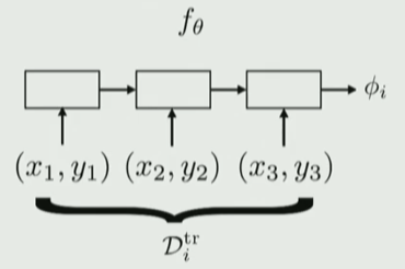
두 번째 NN
또 다른 Neural Network를 사용하여 prediction
요약 : Train with standard Supervised Learning!
- \(\max _{\theta} \sum_{\mathcal{T}_{i}} \sum_{(x, y) \sim \mathcal{D}_{i}^{\text {test }}} \log g_{\phi_{i}}(y \mid x)\).
- \(i\)번째 task 관련 : \(\mathcal{L}\left(\phi_{i}, \mathcal{D}_{i}^{\text {test }}\right)=\sum_{(x, y) \sim \mathcal{D}_{i}^{\text {test }}} \log g_{\phi_{i}}(y \mid x)\).
- 즉, \(\max _{\theta} \sum_{\mathcal{T}_{i}}\mathcal{L}\left(\phi_{i}, \mathcal{D}_{i}^{\text {test }}\right)\).
Algorithm
- Sample task \(\mathcal{T}_{i}\).
-
Split \(\mathcal{D}_{i}\) into \(\mathcal{D}_{i}^{\operatorname{tr}}, \mathcal{D}_{i}^{\text {test }}\) ( Train & Test split )
-
Compute \(\phi_{i} \leftarrow f_{\theta}\left(\mathcal{D}_{i}^{\mathrm{rr}}\right)\).
-
Update \(\theta\) using \(\nabla_{\theta} \mathcal{L}\left(\phi_{i}, \mathcal{D}_{i}^{\text {test }}\right)\)
( where \(\mathcal{L}\left(\phi_{i}, \mathcal{D}_{i}^{\text {test }}\right)=\sum_{(x, y) \sim \mathcal{D}_{i}^{\text {test }}} \log g_{\phi_{i}}(y \mid x)\) )
Challenges
Outputting all NN params… not scalable?
-
모든 output param을 뽑아낼 필요 X ! SUFFICIENT STATISTICS만! (lower dimension vector \(h_i\) )
새로운 param : \(\phi_{i}=\left\{h_{i}, \theta_{g}\right\}\).
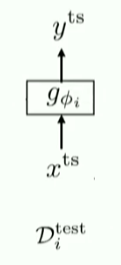
Example Structures
Pros & Cons
Pros
- Expressive
- 다양한 learning problem과 결합 가능
Cons
- 너무 complex
- optimization의 어려움
- data-inefficient ( 매우 큰 meta-tranining data(task)가 필요 )
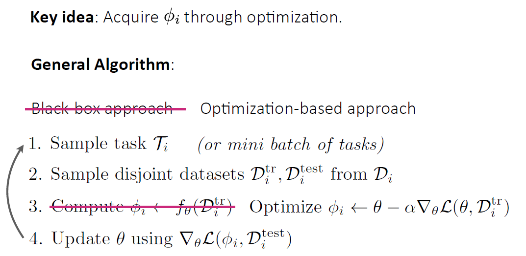
5. Optimization-Based Inference
\(\phi_i\)를 optimization 통해 얻기!
- \(\max _{\phi_{i}} \log p\left(\mathcal{D}_{i}^{\operatorname{tr}} \mid \phi_{i}\right)+\log p\left(\phi_{i} \mid \theta\right)\).
Meta-parameter (\(\theta\))가 PRIOR로써 역할
-
어떻게 prior로써 사용?
Initialization for fine tuninig으로써!
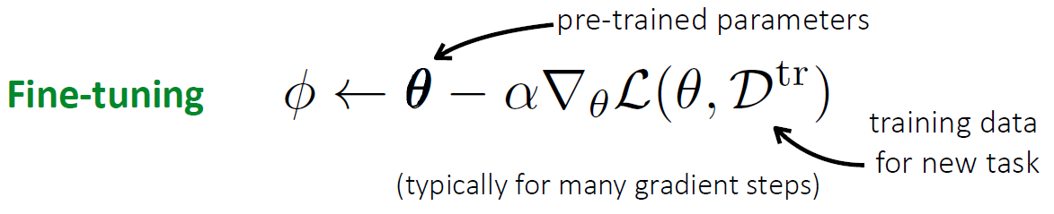
Pre-trained parameter는 어디서?
- (image) ImageNet Classificaiton
- (nlp) BERT, LMs
- (etc) 다른 unsupervised learning techniques
Common practices
- fine tunie with SMALLER learning rate
- lower LR for lower layer
- FREEZE earlier layers & gradually freeze
- REINITIALIZE lats layer
optimization-based Meta Learning 한 줄 요약
- \[\min _{\theta} \sum_{\text {task } i} \mathcal{L}\left(\theta-\alpha \nabla_{\theta} \mathcal{L}\left(\theta, \mathcal{D}_{i}^{\mathrm{tr}}\right), \mathcal{D}_{i}^{\mathrm{ts}}\right)\]
- 모든 task를 사용하여, fine tuning 을 통해 \(\theta\) 얻어내기!
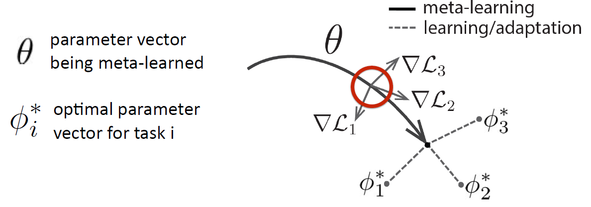
- Model-Agnostic Meta-Learning이라고도 부름!
Algorithm
6. Black-Box Adaptation vs Optimization
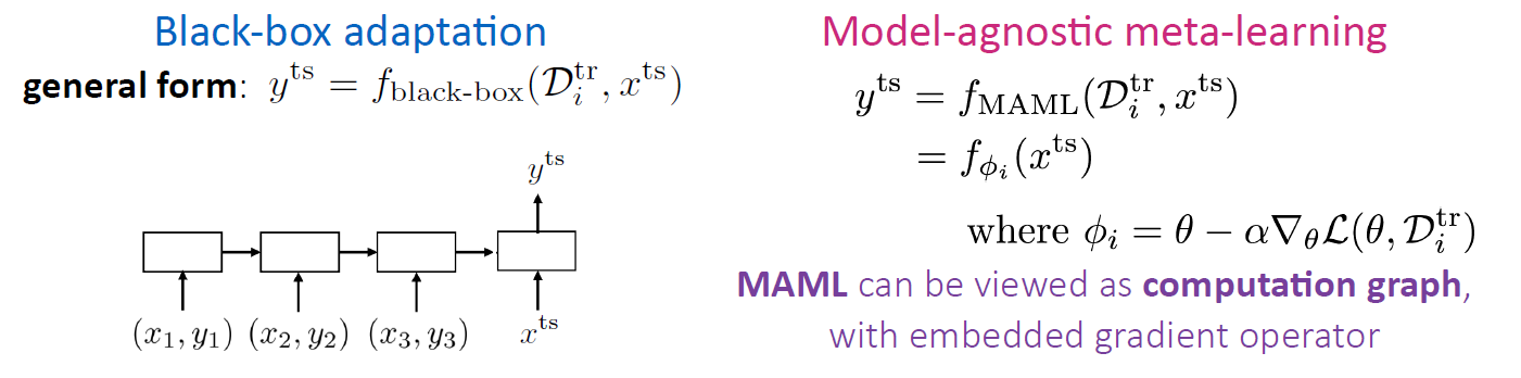
둘을 섞어서 사용할 수 있음!
- 1) “Learn Initialization”
- 2) replace gradient update with “Learned Network”
- before ) \(\begin{array}{r} \phi_{i}=\theta-\alpha \nabla_{\theta} \mathcal{L}\left(\theta, \mathcal{D}_{i}^{\mathrm{tr}}\right) \\ \end{array}\)
- after ) \(\phi_{i}=\theta-\alpha f\left(\theta, \mathcal{D}_{i}^{\mathrm{tr}}, \nabla_{\theta} \mathcal{L}\right)\)
성능 비교
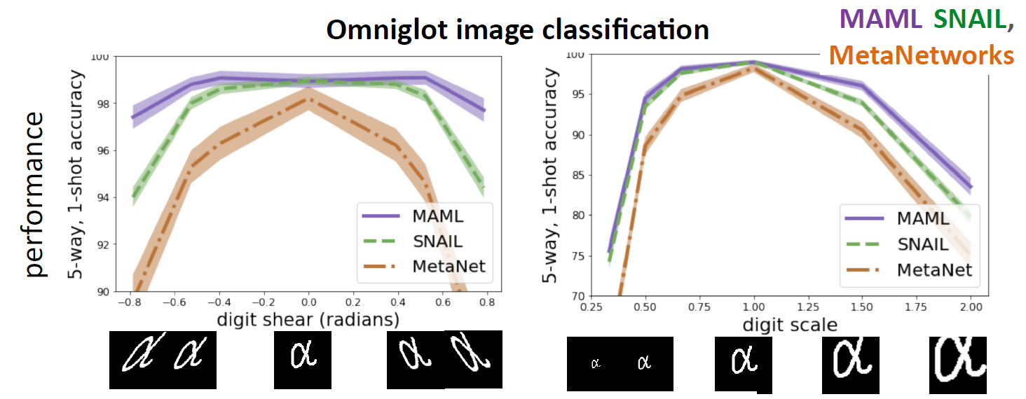
- (MAML) 매우 deep하면, 어떠한 함수든 approximate 가능
- MAML has benefit of inductive bias, without losing expressive power!