[meta] (paper 7) Learning to Propagate Labels ; Transductive Propagation Network for Few shot Learning

Learning to Propagate Labels : Transductive Propagation Network for Few shot Learning

Contents

1. Abstract
2. Introduction
3. Related Works
   1. Meta Learning
   2. Embedding & Metric Learning approaches
   3. Transduction
4. Main Approach
   1. Problem Definition
   2. Transductive Propagation Network (TPN)
      1. Feature Embedding
      2. Graph Construction
      3. Label Propagation
      4. Classification Loss Generation

0. Abstract

Few-shot learning의 목표 :

• learn a (1) classifier
• that (2) generalizes well
• even when trained with a (3) limited number of training instances per class

이 논문에서는 이를 풀기 위한 TPN을 제안

Transductive Propagation Network (TPN)

• classify entire test set AT ONCE

• learn to propagate labels

  • labeled instances \(\rightarrow\) unlabeled test instances

    ( 방법 : graph construction module …. 데이터의 manifold structure를 찾아내! )

• jointly learn (1) & (2)

  • (1) parameters of feature embedding
  • (2) graph construction

• end-to-end

1. Introduction

DL은 large amount of labeled data에 매우 의존적

• 그렇지 않으면, over-fitting issue
• Vinyal et al (2016)
  • propose meta-learning strategy
  • learns over diverse classification tasks, over large number of episodes
  • 각 episode :
    • Support set으로 embedding 학습
    • Unlabeled 데이터인 Query set으로 prediction
  • episode training 방식으로 하는 이유 : test & train 상황 맞추기 위해!

Fundamental difficulty

• 아무리 episode training 방식이 few-shot learning에 맞춤형이라 하더라도, 본질적인 scarce data problem은 어쩔 수 없다.

• 이를 해결하기 위해, consider relationships between instances in the test set

  \(\rightarrow\) 이들을 통채로(as a whole) 예측한다! 이를 TRANSDUCTION (혹은 transductive inference)라고 한다

Transductive inference

• outperform inductive method

  ( inductive : one-by-one prediction )

• 대표적 방법 : construct network on BOTH labeled & unlabeled data

  그런 뒤, propagate labels!

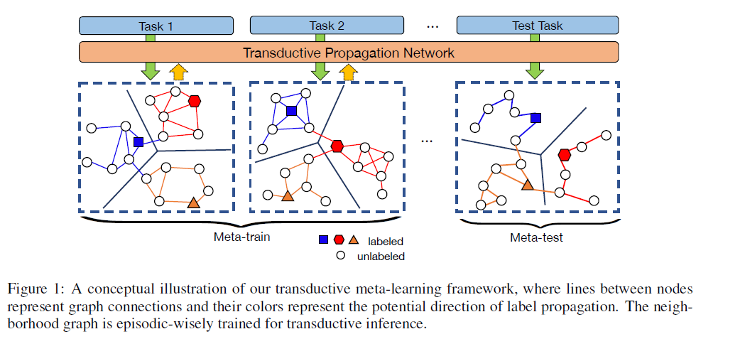
Transductive Propagation Network (TPN)

핵심 특징들

• deal with low-data problem
• transductive inference를 위해 ENTIRE query set을 사용한다

알고리즘 개요

• step 1) DNN 사용하여 embedding space로 input을 mapping
• step 2) graph construction module을 사용하여 manifold structure를 잡아낸다

Main Contribution

• 1) few-shot learning에 transductive inference를 expliclitly하게 model한 최초 알고리즘

  ( 기존에 Nichol et al (2018)에서 제안했던 방법 : only share information between text examples by BN )

• 2) propose to learn to propagate labels

2. Related Works

(a) Meta-learning

• tries to optimize over..
  • batches of tasks (O)
  • batches of data points (X)
• [alg 1] MAML
  • find more transferable representations with “sensitive” parameters
• [alg 2] Reptile
  • first-order meta-learning approach
  • FOMAML (first-order MAML) 와 유사, but train-test split 안해

위 두 알고리즘에 비해, TPN는 closed-form solution for label propagation on query points

\(\rightarrow\) inner update에서 gradient computation 불필요

(b) Embedding & Metric Learning approaches

few-shot learning을 푸는 또 다른 방법 : metric learning approaches

• [alg 1] Matching Networks

  • support set 사용하여 weighted nearest neighbor classifier 학습

  • adjust feature embedding

    ( according to the performance on the query set )

• [alg 2] Prototypical Networks

  • class 별 prototype을 계산 ( = mean of support set)

• [alg 3] Relation Network

  • learn a deep distance metric to compare a small number of images within episodes

(c) Transduction

• [alg 1] Transductive Support Vector Machines (TSVMs)
  • margin-based classification
  • minimize errors of particular test set
• [alg 2] Label Propagation
  • transfer labels ( labeled \(\rightarrow\) unlabeled )
  • guided by weighted graph
• [alg 3] NIchol et al (2018)
  • few shot learning에 transductive setting 적용
  • BUT, only share information between “test examples” via BN

3. Main Approach

주어진 few-shot classification task의 manifold structure를 활용한다!

3-1. Problem Definition

Dataset

• \(\mathcal{C}_{\text {train }}\) : Large + Labeled
• \(\mathcal{C}_{\text {test }}\) : 오직 일부만이 Labeled ( 대부분 Unlabeled )

Episode

• step 1) sample small subset of \(N\) classes from \(\mathcal{C}_{\text {train }}\)

• step 2) 여기서 뽑힌 데이터를 support & query set으로 나눔

  • (1) support set : \(K\) examples from \(N\) classes ( = N-way K-shot learning )

    \[\mathcal{S}=\left\{\left(\mathbf{x}_{1}, y_{1}\right),\left(\mathbf{x}_{2}, y_{2}\right), \ldots,\left(\mathbf{x}_{N \times K}, y_{N \times K}\right)\right\}.\]
    • episode 내에서 training set의 역할을 함

  • (2) query set : support set과는 다른 데이터 ( class는 똑같아 )

    \(\mathcal{Q}=\left\{\left(\mathrm{x}_{1}^{*}, y_{1}^{*}\right),\left(\mathrm{x}_{2}^{*}, y_{2}^{*}\right), \ldots,\left(\mathrm{x}_{T}^{*}, y_{T}^{*}\right)\right\}\).

    • episode 내에서 query set에 대한 loss를 minimize하도록 학습

episodic training을 사용한 Meta-learning 방법들은 few-shot classification 문제에서 잘 작동한다.

하지만, 여전히 lack of labeled instances! (\(K\)로는 부족해….)

\(\rightarrow\) Transductive setting을 사용하게끔 하는 배경!

3-2. Transductive Propagation Networks (TPN)

4개의 구성 요소

1. Feature embedding ( with CNN )
2. Graph construction
   • example-wise parameters to exploit manifold structure
3. Label propagation : \(\mathcal{S} \rightarrow \mathcal{Q}\)
4. Loss generation
   • \(\mathcal{Q}\)에 대해, propagated label & ground 사이의 Cross Entropy loss 계산

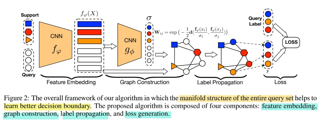
(a) Feature Embedding

• feature extraction 위해 CNN \(f_{\varphi}\) 사용
• \(f_{\varphi}\left(\mathrm{x}_{i} ; \varphi\right)\) : feature map
• SAME embedding function \(f_{\varphi}\) for both \(\mathcal{S}\) & \(\mathcal{Q}\).

(b) Graph Construction

(1) Manifold learning이란?

• discovers the embedded LOW-dimensional subspace in the data

• critical to choose an appropriate neighborhood graph.

• 자주 사용하는 function :

  Gaussian similarity function : \(W_{i j}=\exp \left(-\frac{d\left(\mathrm{x}_{i}, \mathrm{x}_{j}\right)}{2 \sigma^{2}}\right)\)

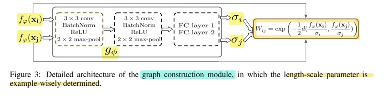
(2) Example-wise length-scale parameter, $\sigma_i$.

• proper neighborhood graph를 얻기 위해, UNION set of \(\mathcal{S} \& \mathcal{Q}\)를 사용한다

• \(\sigma_{i}=g_{\phi}\left(f_{\varphi}\left(\mathrm{x}_{i}\right)\right)\).

  • \(g_{\phi}\) : CNN
  • \(f_{\varphi}\left(\mathrm{x}_{i}\right)\) : input으로 들어가는 feature map

• 이렇게 생성된 example-wise length-scale parameter인 \(\sigma_i\)는,

  아래 similarity function에 input!

  \(W_{i j}=\exp \left(-\frac{1}{2} d\left(\frac{f_{\varphi}\left(\mathrm{x}_{\mathrm{i}}\right)}{\sigma_{i}}, \frac{f_{\varphi}\left(\mathrm{x}_{\mathrm{j}}\right)}{\sigma_{j}}\right)\right)\)….. \(W \in R^{(N \times K+T) \times(N \times K+T)}\).

• 이렇게 해서 나온 \(W\)에 normalized graph Laplacians을 적용 ( \(S=D^{-1/2}WD^{-1/2}\) )

(3) Graph Construction structure

(4) Graph Construction in each episode

• graph is INDIVIDUALLY constructed for EACH TASK in EACH EPISODE

  ( 위의 figure 1 참조 )

• ex) 5-way 5-shot training ( \(N=5, K=5, T=75\) )

  \(\rightarrow\) \(W\)는 고작 100 x 100 차원 ( 꽤 efficient )

(c) Label Propagation

How to get predictions for \(\mathcal{Q}\) using label propagation?

Notation

• \(\mathcal{F}\) : \((N \times K+T) \times N\) matrix with non-neg entries
  • \(N \times K\) 개의 Support Set & \(T\)개의 Query Set
• label matrix \(Y \in \mathcal{F}\)
  • \(Y_{i j}=1\) ……… if \(\mathbf{x}_{i}\) is from the support set & labeled as \(y_{i}=j\),
  • \(Y_{i j}=0\) ……… otherwise ( = label이 없거나, 틀리거나 )

\(Y\)에서 시작해서, iterative하게 determine

• \[F_{t+1}=\alpha S F_{t}+(1-\alpha) Y\]
  • \(S\)는 normalized weight
  • \(\alpha\)는 얼마나 propagate 조절할지 결정
• [최종] closed form solution : \(F^{*}=(I-\alpha S)^{-1} Y\)

Time complexity :

• matrix inversion : \(O(n^3)\)
• 하지만, 여기서 \(n = N \times K + T\) … 매우 작다! efficient

(d) Classification Loss Generation

다음 둘 ( \(F^{*}\) & ground truth )의 차이를 loss로 계산

• 1) \(F^{*}\) : predictions of the \(\mathcal{S} \cup \mathcal{Q}\) ( via label propagation )
• 2) ground truth

\(F^{*}\)는 softmax를 통해 probabilistic score로 변환된다.

• \(P\left(\tilde{y}_{i}=j \mid \mathbf{x}_{i}\right)=\frac{\exp \left(F_{i j}^{*}\right)}{\sum_{j=1}^{N} \exp \left(F_{i j}^{*}\right)}\).

Loss Function :

• \(J(\varphi, \phi)=\sum_{i=1}^{N \times K+T} \sum_{j=1}^{N}-\mathbb{I}\left(y_{i}==j\right) \log \left(P\left(\tilde{y}_{i}=j \mid \mathbf{x}_{i}\right)\right)\).