[cs330] (4강) Non-parametric Meta-Learners

Non-parametric Meta-Learners

Standford CS330 수강 후 강의 내용 요약

1. [RECAP] Optimization-based ML

Fine Tuning : \(\phi \leftarrow \theta-\alpha \nabla_{\theta} \mathcal{L}\left(\theta, \mathcal{D}^{\mathrm{tr}}\right)\).

• ex) MAML (Model Agnostic Meta Learning)

  \(\min _{\theta} \sum_{\text {task } i} \mathcal{L}\left(\theta-\alpha \nabla_{\theta} \mathcal{L}\left(\theta, \mathcal{D}_{i}^{\mathrm{tr}}\right), \mathcal{D}_{i}^{\mathrm{ts}}\right)\).

  • held-out dataset에 얼마나 좋은 performance를 보였는지에 따라 fine-tune

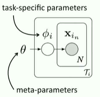
Probabilistic Interpretation of Optimization-based Inference

Optimization-based Inference :

• 핵심 : \(\phi_i\)를 optimization을 통해 구하자

Probabilsitic Interpretation :

• meta parameter인 \(\theta\)는 PRIOR로써의 역할

  ( ex. initialization, fine-tuning )

• .

\[\begin{array}{l} \max _{\theta} \log \prod p\left(\mathcal{D}_{i} \mid \theta\right) \\ \quad=\log \prod_{i} \int p\left(\mathcal{D}_{i} \mid \phi_{i}\right) p\left(\phi_{i} \mid \theta\right) d \phi_{i} \\ \quad \approx \log \prod_{i} p\left(\mathcal{D}_{i} \mid \hat{\phi}_{i}\right) p\left(\hat{\phi}_{i} \mid \theta\right) \end{array}\]

where \(\hat{\phi}_{i}\) is MAP estimate

[ MAP estimate 구하는 방법 ]

“GD with early stopping” = “MAP” under Gaussian prior, with mean at initial params

( exact in linear case, approximate in non-linear case)

즉, MAML approximates Hierarchical Bayesian Inference!!!

Gaussian Prior말고 다른 prior는?

• GD with explicit Gaussian prior :
  • \(\phi \leftarrow \min _{\phi^{\prime}} \mathcal{L}\left(\phi^{\prime}, \mathcal{D}^{\mathrm{tr}}\right)+\frac{\lambda}{2}\left\|\theta-\phi^{\prime}\right\|^{2}\).
• Bayesian Linear Regression on learned features
• Closed-form or Convex Optimization on learned features

Challenges of Optimization-based method

Challenge 1 : “inner-gradient step를 effective하게 할 architecture 찾기!”

“AutoMeta (Kim et al., 2018)”

• IDEA : Progressive Neural Architecture Search + MAML
• highly non-standard architecture ( deep & narrow )
• https://arxiv.org/abs/1806.06927 읽어보기!

Challenge 2 : “Bi-level optimization으로 인한 instability”

“MetaSGD (Li et al.)”, “AlphaMAML(Behl et al.)”

• inner vector learning rate를 자동으로 학습 & outer learning rate를 tune

“DEML (Zhou et al.)”, “CAVIA (Zintgraf et al.)”

• inner loop에서, parameter 중 일부(subset)만 optimize

“MAML++ (Antoniou et al.)”

• decouple inner learning rate
• BN statistics per-step

“Bias transformation (Finn et al.)”, “CAVIA (Zintgraf et al.)”

• context variable 도입으로 more expressive

Challenge 3 : “Backprop through many inner gradient steps의 메모리/연산량 problem”

“first-order MAML (Finn et al.)”, “Reptile (Nichol et al.)”

• \(\frac{d \phi_{i}}{d \theta}\)를 identity로 근사
• 단점 ) simple한 few-shot problem에는 잘 되지만, complex problem에는 X

Second-order optimization을 해야 하는 경우가 일반적! 이를 해결하기 위해, “NON-parametric methods” 사용!

[ 2. Non-parametric Methods ]

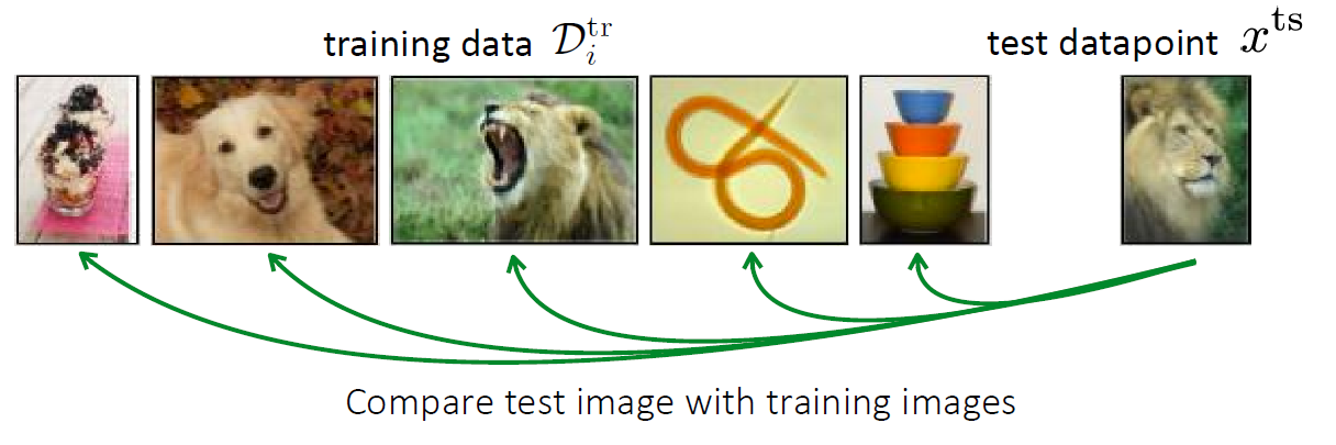
Non-parametric learner 사용하기!

단적인 예로, test-image와 train-image의 거리(유사도) 비교

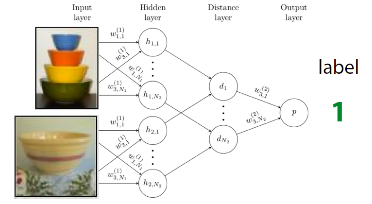
2-1. Siamese Network

Siamese Neural Networks for One-shot Image Recognition

[ Meta-Train 단계 ] : Binary Classification

• Siamese Network를 학습시켜서, 두 image가 같은지 여부 학습

• .

[ Meta-Test 단계 ] : N-way Classification

• \(X_{test}\)를 \(D_j^{tr}\)의 모든 image와 비교

Meta-Train와 Meta-Test를 match하는 것이 point!

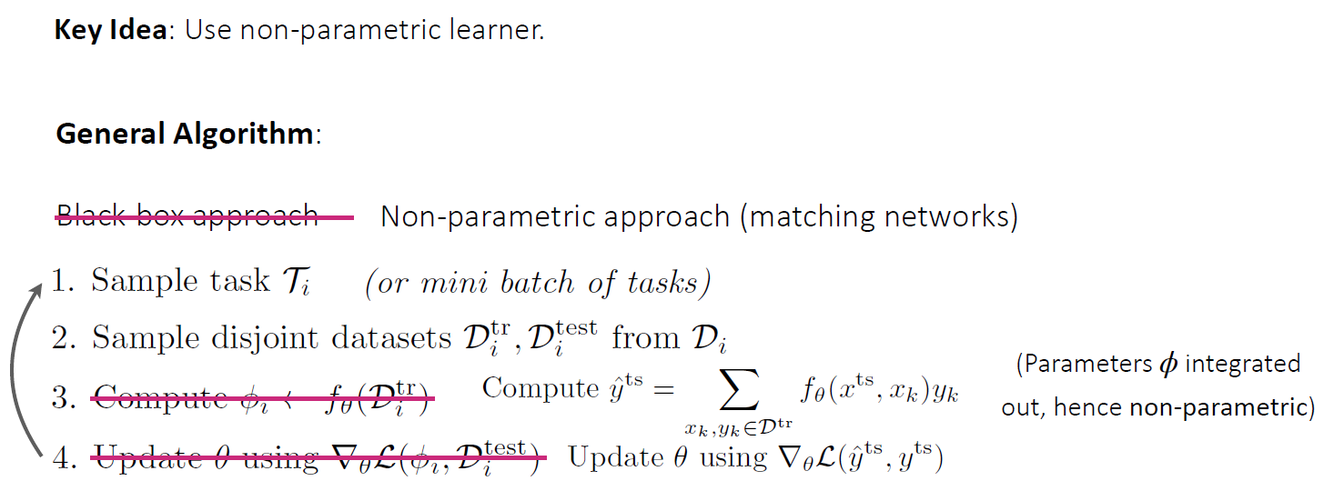
2-2. Matching Network

Matching Networks for One Shot Learning

• train & test 데이터 모두 같은 embedding space로 embed
• 사용 모델
  • bidirectional LSTM
  • Convolutional Encoder
• end-to-end 모델

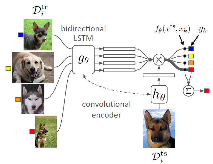
• \(\hat{y}^{\mathrm{ts}}=\sum_{x_{k}, y_{k} \in \mathcal{D}^{\operatorname{tr}}} f_{\theta}\left(x^{\mathrm{ts}}, x_{k}\right) y_{k}\).

Algorithm

2-3. Prototypical Network

Prototypical Networks for Few-shot Learning

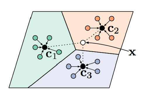
class 별 centroid 찾고, 거리(euclidean 혹은 cosine)비교하여 class 판별

• centroid : \(\mathbf{c}_{n}=\frac{1}{K} \sum_{(x, y) \in \mathcal{D}_{i}^{\mathrm{rr}}} \mathbb{1}(y=n) f_{\theta}(x)\).

Prediction

• \(p_{\theta}(y=n \mid x)=\frac{\exp \left(-d\left(f_{\theta}(x), \mathbf{c}_{n}\right)\right)}{\sum_{n^{\prime}} \exp \left(d\left(f_{\theta}(x), \mathbf{c}_{n^{\prime}}\right)\right)}\).

3. Challenges of Non Parametric Models

data point 사이의 더 complex relationship을 잡아내고 싶으면?

이를 해결 하기 위해 고안된…

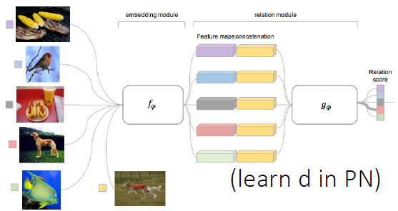
3-1. Relation Net

Learning to Compare: Relation Network for Few-Shot Learning

• learn “non-linear” relation module on embeddings

3-2. Infinite Mixture Prototypes

Infinite Mixture Prototypes for Few-Shot Learning - arXiv

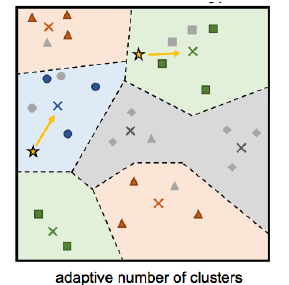
• learn infinite mixtures of prototypes

3-3. Graph Neural Networks

Few-Shot Learning with Graph Neural Networks

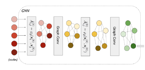
• ‘Message Passing’ on embeddings

4. Black-box vs Optimization vs Non-parametric

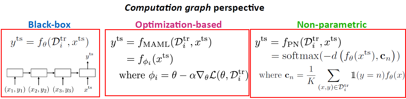
위의 것들을 서로 mix하여 사용할 수 있음!

Examples

Learning to Learn with Conditional Class Dependencies …

• Both condition on data & run GD

Meta-Learning with Latent Embedding Optimization

• Gradient descent on relation net embedding

Meta-Dataset: A Dataset of Datasets for Learning to Learn …

• MAML + initialize last layer as ProtoNet during meta-training

Pros & Cons

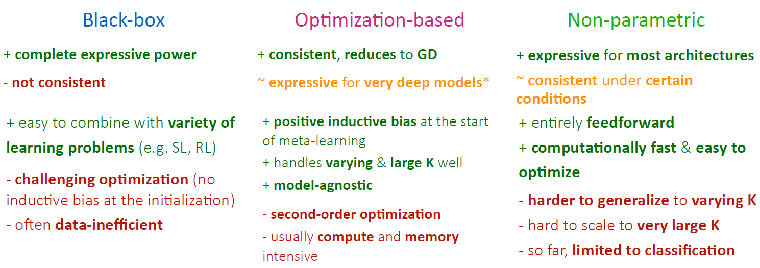
Summary : 3 가지 중요한 특징

• 1) Expressive Power ( for scalability & applicability )

• 2) Consistency ( 데이터 \(\uparrow\) 수록 성능 \(\uparrow\) , meta-training task에 rely 적어야, OOD에 좋은 성능 )

• 3) Uncertainty Awareness ( uncertainty 측정 가능 여부 )