
Learning to Compare : Relation Network for Few-shot Learning (2018)
Contents
- Abstract
- Introduction
- Methodology
- Problem Definition
- Model
- Zero-shot Learning
- Network Architecture
0. Abstract
Simple & Flexible & General framework for few-shot learning인 “RELATION NETWORK (RN)”을 제안함
Step 1) Meta Learning 중..
- learns to learn a “deep distance metric”
Step 2) Once trained…
-
classify image of NEW classes by computing “relation scores” between
(1) query images & (2) few examples of each new class ( = from support images)
1. Introduction
train an “effective metric” for one-shot learning!
aim to learn a transferable deep metric for comparing the relations
- 1) between images ( = few-shot learning )
- 2) between images & class descriptions ( = zero-shot learning )
propose two-branch Relation Network (RN)
- (1) Embedding module
- generates representations of query & training images
- (2) Relation module
- calculate “relation score”
- 해당 category에 match하는지 안하는지 0~1
2. Methodology
2-1. Problem Definition
task : few-shot classifier learning
dataset : 3종류의 데이터 ( train / support / test )
-
support & test : label space를 공유한다 ( class F,G,H,I )
\(\leftrightarrow\) train은 자신만의 label space를 가짐 ( class A,B,C,D,E )
-
support set : \(C\)-way \(K\)-shot
원칙적으로는, 적은양의 데이터만을 가진 Support set을 사용해서 model을 만든 뒤,
Test set의 데이터를 예측할 수는 있음
( BUT… lack of labelled samples in Support Set…. 나쁜 성능! )
따라서, aim to perform meta-learning on “TRAINING SET”,
in order to “EXTRACT TRANSFERRABLE KNOWLEDGE”
이를 풀기 위해 자주 사용되는 “Episode based training”
매 training episode마다…
- random select \(C\) classes with \(K\) examples from TRAINING SET
- sample set ( =support set) \(S\) : \(\mathcal{S}=\left\{\left(x_{i}, y_{i}\right)\right\}_{i=1}^{m}(m=K \times C)\).
- query set \(Q\) : \(\mathcal{Q}=\left\{\left(x_{j}, y_{j}\right)\right\}_{j=1}^{n}\) ( \(K\)개 뽑고 남은거만큼 )
- 위 두 sample & query set으로 학습한다
- sample set으로 모델 만들고
- query set으로 loss 계산해서 back-prop
2-2. Model
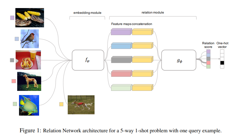
(1) One-shot
- embedding module : \(f_{\varphi}\)
- relation module : \(g_{\phi}\)
- data :
- sample set \(S\) : \(x_{i}\) …… feature map : \(f_{\varphi}\left(x_i\right)\)
- query set \(Q\) : \(x_{j}\) ……… feature map : \(f_{\varphi}\left(x_{j}\right)\)
- concatenate 2 feature maps : \(\mathcal{C}\left(f_{\varphi}\left(x_{i}\right), f_{\varphi}\left(x_{j}\right)\right)\)
-
\(\mathcal{C}\left(f_{\varphi}\left(x_{i}\right), f_{\varphi}\left(x_{j}\right)\right)\) 가 \(g_{\phi}\) 를 지나서 0~1사이 값 (=similarity, relation score) 가 나옴
- relation score :
- \(r_{i, j}=g_{\phi}\left(\mathcal{C}\left(f_{\varphi}\left(x_{i}\right), f_{\varphi}\left(x_{j}\right)\right)\right), \quad i=1,2, \ldots, C\).
- 하나의 query set data \(x_j\)에 대해, 총 \(C\)개 ( =sample set 개수) 만큼의 relation score가 나옴
(2) K-shot
- 위와 동일
- 단지, sample set의 embedding module 결과값을 “element-wise sum”하면 됨
(3) Objective Function
MSE 사용
- \(\varphi, \phi \leftarrow \underset{\varphi, \phi}{\operatorname{argmin}} \sum_{i=1}^{m} \sum_{j=1}^{n}\left(r_{i, j}-\mathbf{1}\left(y_{i}==y_{j}\right)\right)^{2}\).
2-3. Zero-shot Learning
one-shot learning 과
- 유사점 ) “one datum is given to define each class” to recognize
- 차이점 ) contains a semantic class embedding vector \(v_c\) for each support set examples
2개의 heterogeneous embedding module을 사용한다
- 1) query set 용 : \(f_{\varphi_{1}}\)
- 2) support set의 semantic class embedding vector 용 : \(f_{\varphi_{2}}\)
나머지는 동일하다! Relation Score 계산은…
- \(r_{i, j}=g_{\phi}\left(\mathcal{C}\left(f_{\varphi_{1}}\left(v_{c}\right), f_{\varphi_{2}}\left(x_{j}\right)\right)\right), \quad i=1,2, \ldots, C\).
2-4. Network Architecture
대부분의 few-shot learning model들은 4개의 conv block를 embedding module로써 사용한다.
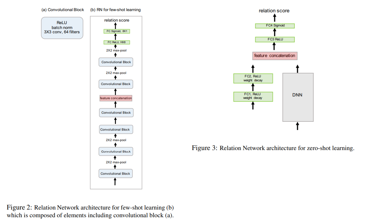
- 여기서 DNN은, pre-trained Network ( ex. Inception / ResNet )으로 ,query set이 input으로 들어가게 된다