
Meta-learning with Latent Embedding Optimization (2019)
Contents
- Abstract
- Introduction
- Methodology
- Problem Definition
- Model
- Zero-shot Learning
- Network Architecture
0. Abstract
Gradient-based Meta-Learning techniques의 어려움 :
- HIGH-dimensional parameter space in LOW-data regimes에서 작동할 때!
이 논문에서는 위의 문제를 다음의 방식으로 극복함
- learn a data-dependent “latent generative representation” of model parameters
- perform gradient-based meta-learning in this “low-dimensional latent space”
\(\rightarrow\) LEO (Latent Embedding Optimization)을 제안한다
1. Introduction
LEO (Latent Embedding Optimization)의 2가지 장점
-
1) Initial parameters for a new task are “conditioned on the training data”,
which enables “task-specific starting point”
-
2) by optimizing in the LOWER-dimensional input, can be done more “EFFICIENTLY”
2. Model
2-1. Problem Definition
Settings & Notation
- 가정 : N-way K-shot
-
task instance \(T_i\)는 task distribution \(p(T)\)에서 sample됨
-
t개의 task : \(T_1\) ,…\(T_t\) ( 이들은 train/valid/test로 구분)
- \(T_1\) ~ \(T_m\) : train task ( training meta-set= \(S^{tr}\) )
- \(T_{m+1} \sim T_n\) : validation task ( validation meta-set= \(S^{val}\) )
- \(T_{n+1} \sim T_{t}\) : test task ( test meta-set= \(S^{test}\) )
-
위의 각 세 세트의 데이터들은, 다음으로 구분
ex) \(S^{tr} = (D^{tr}, D^{val}, D^{test})\)
- \(\mathcal{D}^{t r}=\left\{\left(\mathbf{x}_{n}^{k}, y_{n}^{k}\right) \mid k=1 \ldots K ; n=1 \ldots N\right\}\).
-
헷갈리지 말기!
- \(D^{val}\) : used to “optimize loss function”
- \(S^{val}\) : used for “model selection”
2-2. MAML ( MODEL-AGNOSTIC META-LEARNING )
Goal :
-
aims to find a “single set of params \(\theta\)“,
which uses a “few” optimization steps,
that can be successfully “adapted to any novel task”
Notation
-
task-specific model parameters : \(\theta_{i}^{\prime}\)
-
\(\theta_{i}^{\prime}=\mathcal{G}\left(\theta, \mathcal{D}^{t r}\right)\) ( 여기서 \(\mathcal{G}\) 는 gradient descent & \(D^{tr}\)는 task \(i\)에 해당하는 dataset )
-
task별 updating equation : ( = adaptation procedure )
\(\theta_{i}^{\prime}=\theta-\alpha \nabla_{\theta} \mathcal{L}_{\mathcal{T}_{i}}^{t r}\left(f_{\theta}\right)\).
- \(\alpha\) : can be meta-learned ( ex. Meta-SGD, 2017 )
-
meta parameter의 updating equation :
\(\theta \leftarrow \theta-\eta \nabla_{\theta} \sum_{\mathcal{T}_{i} \sim p(\mathcal{T})} \mathcal{L}_{\mathcal{T}_{i}}^{v a l}\left(f_{\theta_{i}^{\prime}}\right)\).
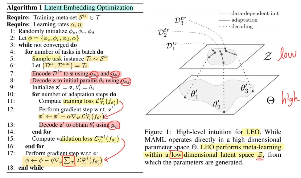
2-3. LEO (Latent Embedding Optimization) for Meta-Learning
high-dimension에서 벗어나서 low-dimension에서 GD가 이루어지면 GOOD!
\(\rightarrow\) achieve this by learning a “STOCHASTIC LATENT SPACE” with an information bottleneck, conditioned on the input data
MAML vs LEO
-
MAML : learn unique set of model parameters \(\theta\)
-
LEO : learn a “generative distribution” of model parameters
(1) Model Overview
Parameter
-
Encoder 부분 : encoder (\(\phi_e\)) + relation network (\(\phi_r\))
- Decoder 부분 : decoder (\(\phi_d\))
- learning rate : \(\alpha\)
- [종합] \(\phi = \phi_e, \phi_r, \phi_d, \alpha\)
Algorithm
Randomly initialize \(\phi_{e}, \phi_{r}, \phi_{d}\) Let \(\phi=\left\{\phi_{e}, \phi_{r}, \phi_{d}, \alpha\right\}\)
given task instance \(T_i\) ( = \((D_{tr}, D_{val}\) ) )
-
step 1) \(D^{tr}\)에 있는 data들 \(\left\{\mathbf{x}_{n}^{k}\right\}\) 는 stochastic encoder에 들어가서 latent code \(\mathbf{z}\)가 나온다
-
step 2) 이 latent code \(\mathbf{z}\)는 다시 decoder로 들어가서 \(\theta_i\)가 나온다 ( using “parameter generator, \(g_{\phi_{d}}\)” )
-
step 3) 이렇게 해서 나온 \(\theta_i\)로 loss 계산 후, \(\mathbf{z}\)의 latent space에서 gradient descent 진행
- \(\mathbf{z}^{\prime} \leftarrow \mathbf{z}^{\prime}-\alpha \nabla_{\mathbf{z}^{\prime}} \mathcal{L}_{\mathcal{T}_{i}}^{t r}\left(f_{\theta_{i}^{\prime}}\right)\).
-
step 4) 이렇게 update된 \(\mathbf{z}^{'}\)를 다시 decoder로 들어가서 \(\theta_i^{'}\)가 나온다 ( using “parameter generator, \(g_{\phi_{d}}\)” )
-
step 2) ~ step 4)를 여러 번 반복한다
-
여러번 반복 뒤, 나오게 된 \(\theta^{'}\)를 사용하여 validation loss \(\mathcal{L}_{\mathcal{T}_{i}}^{v a l}\left(f_{\theta_{i}^{\prime}}\right)\) 계산
이 loss를 사용하여 \(\phi\)를 update한다.
\(\phi \leftarrow \phi-\eta \nabla_{\phi} \sum_{\mathcal{T}_{i}} \mathcal{L}_{\mathcal{T}_{i}}^{v a l}\left(f_{\theta_{i}^{\prime}}\right)\).
(2) Initialization : Generating Parameters Conditioned on a few examples
stage 1) instantiate model parameters, that will be adapted to each task instance
-
MAML : single set of model params
-
LEO : data-dependent latent encoding ( 추후 decoded to generate actual initial params )
( = consider context, when producing parameter initial params )
Encoding
2개의 과정을 거쳐서 encoding 된다
- encoder network : \(g_{\phi_{e}}: \mathcal{R}^{n_{x}} \rightarrow \mathcal{R}^{n_{h}}\)
- relation network : \(g_{\phi_{r}}\)
\(K\)-shot training samples, corresponding to each class \(n\)
- \(n: \mathcal{D}_{n}^{t r}=\left\{\left(\mathbf{x}_{n}^{k}, y_{n}^{k}\right) \mid k=\right.1 \ldots K\}\).
Encoding 과정
( class별로 생성한다! class-dependent codes : \(\mathbf{z}=\left[\mathbf{z}_{1}, \mathbf{z}_{2}, \ldots, \mathbf{z}_{N}\right]\) )
\(\begin{aligned} \boldsymbol{\mu}_{n}^{e}, \boldsymbol{\sigma}_{n}^{e}=& \frac{1}{N K^{2}} \sum_{k_{n}=1}^{K} \sum_{m=1}^{N} \sum_{k_{m}=1}^{K} g_{\phi_{r}}\left(g_{\phi_{e}}\left(\mathbf{x}_{n}^{k_{n}}\right), g_{\phi_{e}}\left(\mathbf{x}_{m}^{k_{m}}\right)\right) \\ & \mathbf{z}_{n} \sim q\left(\mathbf{z}_{n} \mid \mathcal{D}_{n}^{t r}\right)=\mathcal{N}\left(\boldsymbol{\mu}_{n}^{e}, \operatorname{diag}\left(\boldsymbol{\sigma}_{n}^{e 2}\right)\right) \end{aligned}\).
Decoding
-
decoder network : \(g_{\phi_{d}}: \mathcal{Z} \rightarrow \Theta\)
- use class-specified latent codes to instantiate just the top layer weights of classifier
-
decoding된 결과 : \(\theta_{i}^{\prime}=\left\{\mathbf{w}_{n} \mid n=1 \ldots N\right\}\)
- without requiring the generator to produce very high-dim params
Decoding 과정
( parameterize Gaussian distn with diagonal covariance )
- sample class-dependent parameters \(\mathbf{w}_{n}\)
- \(\begin{aligned} \boldsymbol{\mu}_{n}^{d}, \boldsymbol{\sigma}_{n}^{d} &=g_{\phi_{d}}\left(\mathbf{z}_{n}\right) \\ \mathbf{w}_{n} \sim p\left(\mathbf{w} \mid \mathbf{z}_{n}\right) &=\mathcal{N}\left(\boldsymbol{\mu}_{n}^{d}, \operatorname{diag}\left(\boldsymbol{\sigma}_{n}^{d^{2}}\right)\right) \end{aligned}\).
(3) Adaptation by LEO ( = INNER loop )
-
특정 task \(T_i\) 별로 수행 ( \(\mathbf{z}\)를 update)
-
Cross-Entropy loss 사용
-
\(\mathcal{L}_{\mathcal{T}_{i}}^{t r}\left(f_{\theta_{i}}\right)=\sum_{(\mathbf{x}, y) \in \mathcal{D}^{t r}}\left[-\mathbf{w}_{y} \cdot \mathbf{x}+\log \left(\sum_{j=1}^{N} e^{\mathbf{w}_{j} \cdot \mathbf{x}}\right)\right]\).
-
위 loss를 사용하여 다음의 GD를 수행
\(\mathbf{z}_{n}^{\prime}=\mathbf{z}_{n}-\alpha \nabla_{\mathbf{z}_{n}} \mathcal{L}_{\mathcal{T}_{i}}^{t r}\).
(4) Meta-Training strategy ( = OUTER loop )
-
모든 task \(T_i\)들에 대해서 전부 수행한 뒤 \(\phi\)를 update
-
\(\min _{\phi_{e}, \phi_{r}, \phi_{d}} \sum_{\mathcal{T}_{i} \sim p(\mathcal{T})}\left[\mathcal{L}_{\mathcal{T}_{i}}^{v a l}\left(f_{\theta_{i}^{\prime}}\right)+\beta D_{K L}\left(q\left(\mathbf{z}_{n} \mid \mathcal{D}_{n}^{t r}\right) \mid \mid p\left(\mathbf{z}_{n}\right)\right)+\gamma \mid \mid \operatorname{stopgrad}\left(\mathbf{z}_{n}^{\prime}\right)-\mathbf{z}_{n} \mid \mid _{2}^{2}\right]+R\).
-
(2번째 term)
weighted KL-div to regularize the latent space & encourage generative model to learn a disentangled embedding
-
(3번째 term)
encourage the encoder & relation net to output a parameter initialization that is close to the adapted code
-