Aspect-based Sentiment Analysis with Type-aware Graph Convolutional Networks and Layer Ensemble (2021)
Contents
- Abstract
- Introduction
- The Approach
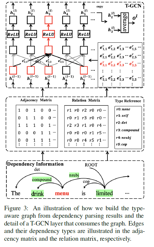
- Type-aware Graph Construction
- T-GCN
- Attentive Layer Ensemble (ALE)
- Encoding & Decoding with T-GCN
0. Abstract
ABSA에 neural graph-based models를 사용하는 경우가 많음
하지만, 대부분의 이러한 연구들은…
- (문제 1) only leverage dependency relations, WITHOUT CONSIDERING DEPENDENCY TYPE
- (문제 2) limited in LACKING EFFICIENT MECHANISM to distinguish important relations
따라서, 아래와 같은 알고리즘을 제안함
explicitly utilize DEPENDENCY TYPES for ABSA with T-GCN
- T-GCN = Type-aware GCN
- attention을 사용하여 edge간의 차이를 구분함!
- attentive layer ensemble을 통해, T-GCN 여러 다른 layer들을 모두 고려
1. Introduction
요즈음 GCN (Graph Convolutional Network)를 자주 사용함
-
(장점) built over dependency parsing results of input text
\(\rightarrow\) 따라서, 문장 내에 멀리 떨어진(distant) 단어도 고려 O
-
(단점 1) dependency type고려 못해
- 즉, node&node가 연결되어 있다하더라도, 중요한 edge인지 아닌지 구분 X
example)
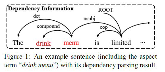
-
menu와 관련있는 단어는 3개 ( The, drink,limited )
-
하지만 이 중 제일 중요한 것은 menu & limited의 dependency
( dependency type = “nsubj” …. 의미 : menu is the nominal subject of limited )
-
-
이러한 dependency type을 고려하지 않는다면, 뭐가 중요한지 파악하기 어려움!
-
(단점 2) Last Layer의 output만을 사용한다
- 즉, intermediate layer의 정보는 손실!
위의 2가지 단점들을 극복하기 위해.. T-GCN with multiple layer를 제안함
-
incorporate both word relations & dependency types
-
알고리즘 순서
-
1) obtain dependency parsing results of the input texts
-
2) build the graph over dependency tree
-
3) apply attention mechanism to graph
-
4) use attentive layer ensemble to weight & combine contextual information
learned from different GCN layers
-
2. The Approach
Notation
- input 문장 : \(\mathcal{X}=x_{1}, x_{2}, \cdots, x_{n}\mathcal{X}=x_{1}, x_{2}, \cdots, x_{n}\)
- aspect term : \(\mathcal{A} \subset \mathcal{X}(\mathcal{A}\)는 주로 문장의 sub-string이다)
- 예측한 sentiment : \(\widehat{y}\)
기존의 ABSA approach는,
- input : sentence-aspect pair
- output : \(\widehat{y}\) ( of aspect )
여기서 제안한 알고리즘을 한줄로 표현하자면…
\(\widehat{y}=\underset{y \in \mathcal{T}}{\arg \max } p(y \mid A L E(T-G C N(\mathcal{X}, \mathcal{A})))\).
- contextual encoder : BERT
- attentive layer ensemble : ALE
논문 설명(소개) 순서
- 1) graph를 construct하는 방법 ( with dependency type )
- 2) T-GCN 모델 & ALE 을 구체화
- 3) T-GCN을 ABSA에 Incorporate하는 방법
2-1) Type-aware Graph Construction
GCN 모델은 contextual features를 잡아내는것에 effective
- ex) dependencies among words
기존의 GCN models
-
두 단어 \(x_i\), \(x_j\) 사이의 edge는 graph에 추가된다 ( 연결되어 있다면 )
( 하지만, dependency type는 추가하지 않아 )
-
따라서 이 논문은 TYPE-AWARE graph를 제안함
-
아래의 step을 따른다
Step 1) dependency result를 얻어낸다
-
즉, dependency tuple \((x_i, x_j, r_{i,j})\)를 얻어낸다
( 여기서 \(r_{i,j}\) 는 dependency type )
Step 2) adjacency matrix \(\mathbf{A}\) & relation type matrix \(\mathbf{R}\) 를 얻어낸다
- \(\mathbf{A}=\left\{a_{i, j}\right\}_{n \times n}\).
- \(\mathbf{R}=\left\{r_{i, j}\right\}_{n \times n}\).
Step 3) relation type를 고려하기 위해, transition matrix를 사용
- use transition matrix to map all \(r_{i,j}\) to their embeddings \(\mathbf{e}_{i,j}^r\)
2-2) T-GCN
L-layer T-GCN을 제안함
-
각 layer에 attention 적용
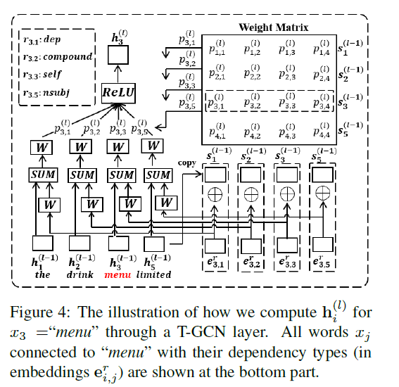
-
두 node 사이의 edge는 (1) hidden vector 뿐만 아니라, (2) embeddings of dependency types를 고려한다
- Step 1)
- \(\mathbf{s}_{i}^{(l)}=\mathbf{h}_{i}^{(l-1)} \oplus \mathbf{e}_{i, j}^{r}\).
- \(\mathbf{s}_{j}^{(l)}=\mathbf{h}_{j}^{(l-1)} \oplus \mathbf{e}_{i, j}^{r}\).
- Step 2-1) 위 두 노드의 edge의 weight 계산
- \(p_{i, j}^{(l)}=\frac{a_{i, j} \cdot \exp \left(\mathbf{s}_{i}^{(l)} \cdot \mathbf{s}_{j}^{(l)}\right)}{\sum_{j=1}^{n} a_{i, j} \cdot \exp \left(\mathbf{s}_{i}^{(l)} \cdot \mathbf{s}_{j}^{(l)}\right)}\).
- Step 2-2)
- \(\mathbf{h}_{j}^{(l-1)^{\prime}}=\mathbf{h}_{j}^{(l-1)}+\mathbf{W}_{R}^{(l)} \cdot \mathbf{e}_{i, j}^{r}\).
- Step 3) 위 weight를 edge에 적용
- \(\mathbf{h}_{i}^{(l)}=\sigma\left(\sum_{j=1}^{n} p_{i j}\left(\mathbf{W}^{(l)} \cdot \mathbf{h}_{j}^{(l-1)^{\prime}}+\mathbf{b}^{(l)}\right)\right)\).
- Step 1)
2-3) Attentive Layer Ensemble (ALE)
multiple T-GCN layers could learn indirect word relations from long distances
( different layers = unique capacities )
Step 1) 각 T-GCN layer로부터 output \(o^{l}\)을 얻어낸다.
- \(\mathbf{o}^{(l)}=\frac{1}{ \mid \mathcal{A} \mid } \cdot \sum_{x_{k} \in \mathcal{A}} \mathbf{h}_{k}^{(l)}\).
Step 2) 이것을 모든 layer들로부터 얻어낸 뒤, weighted average한다.
-
\(\mathbf{o}=\sum_{l=1}^{L} \delta^{(l)} \cdot \mathbf{o}^{(l)}\).
( \(\sum_{l=1}^{L} \delta^{(l)}=1\) )
2-4) Encoding & Decoding with T-GCN
Encoding
2가지 방법이 있다.
- 방법 1) \(\mathbf{H}^{\mathcal{X}}=B E R T(\mathcal{X})\) …. sentence만을 input으로
- 방법 2) \(\left[\mathbf{H}^{\mathcal{X}}, \mathbf{H}^{\mathcal{A}}\right]=\operatorname{BERT}(\mathcal{X}, \mathcal{A})\) …… sentence-aspect pair를 input으로
- \(\mathbf{H}^{\mathcal{A}}\) : hidden vectors of all aspect words
Decoding
ALE (Attentive Layer Ensemble)로부터 \(\mathbf{o}\)를 얻어낸 뒤, map \(\mathbf{o}\) to the label space ( with FC layer )
- \(\mathbf{u}=\mathbf{W} \cdot \mathbf{o}+\mathbf{b}\).
- 최종 output : \(\hat{y}=\arg \max \frac{\exp \left(u^{t}\right)}{\sum_{t=1}^{ \mid \mathcal{T} \mid } \exp \left(u^{t}\right)}\).