
Model-Agnostic Meta-Learning for Fast Adaptation of Deep Networks
Contents
- Abstract
- Introduction
- Model-Agnostic Meta-Learning (MAML)
- Meta-Learning Problem Set-up
- MAML algorithm
- 기타
- Multi-task vs Meta Learning
- Meta-Learning Approaches
0. Abstract
Key Point 요약
- 1) Model-Agnostic한 meta-learning 알고리즘을 제안
- 2) small number of training samples에서도 좋은 성능을 내도록!
- 3) MAML trains the model to be easy to fine tune
1. Introduction
Learning Quickly! 인간처럼
Meta Learning은 task에 GENERAL해야!
Meta Learning의 목적
-
1) quickly learn new task on small data
-
2) able to learn on large number of different tasks
이 논문이 제안한 MAML은…
-
(1) general : any learning problem
-
(2) model-agnostic : any **model **( GD 사용하는 model이면 OK )
-
parameter 수를 늘리지도 않음 & 모델 architecture 제한도 없음
( 단지 simply fine-tune parameters slightly! )
한 줄 요약 : SMALL number of gradient update만으로도 FAST learning on new task
2. Model-Agnostic Meta-Learning
achieve RAPID adaptation
2-1. Meta-Learning Problem Set-up
few shot learning의 목적 :
-
few data point만으로도, new task에 fast adopt
-
그러기 위해, model(=learner)는
- meta learning phase에서 여러 task를 사용하여 학습됨
- 모든 tasks들을 일종의 training example로써 취급한다
Notation
-
Task : \(\mathcal{T}=\left\{\mathcal{L}\left(\mathbf{x}_{1}, \mathbf{a}_{1}, \ldots, \mathbf{x}_{H}, \mathbf{a}_{H}\right), q\left(\mathbf{x}_{1}\right), q\left(\mathbf{x}_{t+1} \mid \mathbf{x}_{t}, \mathbf{a}_{t}\right), H\right\}\)
-
loss function : \(\mathcal{L}\)
-
distribution over initial observation : \(q\left(\mathbf{x}_{1}\right)\)
-
transition distribution : \(q\left(\mathbf{x}_{t+1} \mid \mathbf{x}_{t}, \mathbf{a}_{t}\right)\)
-
episode length : \(H\)
( 지도학습의 경우 \(H=1\) )
-
-
\(\operatorname{loss} \mathcal{L}\left(\mathrm{x}_{1}, \mathbf{a}_{1}, \ldots, \mathrm{x}_{H}, \mathbf{a}_{H}\right) \rightarrow \mathbb{R}\) : task-specific feedback을 준다
( ex. mis-classificaiton loss, cost function in MDP )
-
distribution over tasks : \(P(\mathcal{T})\)
Metal Training 과정
-
1) task를 샘플한다 ….. \(T_i \sim p(T)\)
-
2) 해당 task의 meta-train data \(\mathcal{D}_{i}^{\text {tr }}\) ( \(K\)개 ) 로 loss (\(L_{T_i}\)) 계산 후 train
- \[\phi_{i} \leftarrow f_{\theta}\left(\mathcal{D}_{i}^{\mathrm{rr}}\right)\]
-
3) meta-test data ( \(\mathcal{D}_{i}^{\text {test }}\) )로 update
-
Update \(\theta\) using \(\nabla_{\theta} \mathcal{L}\left(\phi_{i}, \mathcal{D}_{i}^{\text {test }}\right)\)
where \(\left.\mathcal{L}\left(\phi_{i}, \mathcal{D}_{i}^{\text {test }}\right)=\sum_{(x, y) \sim \mathcal{D}_{i}^{\text {test }}} \log g_{\phi_{i}}(y \mid x)\right)\)
-
위의 Meta Train이 다 끝나고 나면, \(P(\mathcal{T})\)에서 새로운 task sample을 뽑은 뒤 해당 task data로 성능 평가!
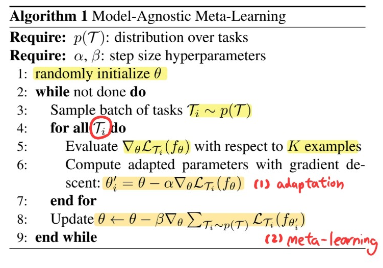
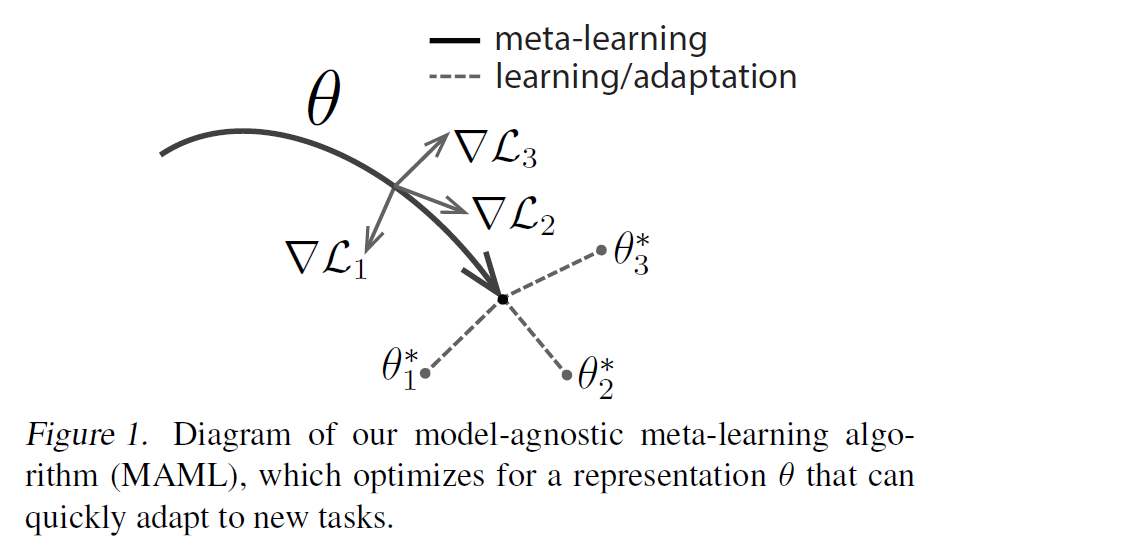
2-2. MAML algorithm
나중가서 model이 새로운 task에 알맞게 fine-tune 될 것이기 때문에,
aim to learn a model in a way that gradient-based learning rule can make RAPID PROGRESS on NEW TASKS drawn from \(p(\mathcal{T})\)
\(\rightarrow\) task의 변화에 따라 SENSITIVE한 model parameter를 찾기!
( sensitive = small change in param \(\rightarrow\) large improvement on loss function )
알고리즘 소개
model : \(f_{\theta}\)
- 위 모델이 새로운 task \(\mathcal{T_i}\)에 adapt하면, \(\theta\) \(\rightarrow \theta^{'}\)
2가지 step으로 구성
-
1) adaptation
-
새로 들어오는 task(데이터)에 맞게 \(\theta\)를 변경(update)하기
( 모든 task들의 initialization은 \(\theta\)로하고, 각자 task에 맞게 \(\theta_i\)로 update )
-
-
2) meta-learning
- \(D_{meta-train}\)을 사용하여 \(\theta\)를 빠르게 update하는 “법”을 배우기
3. Species of MAML
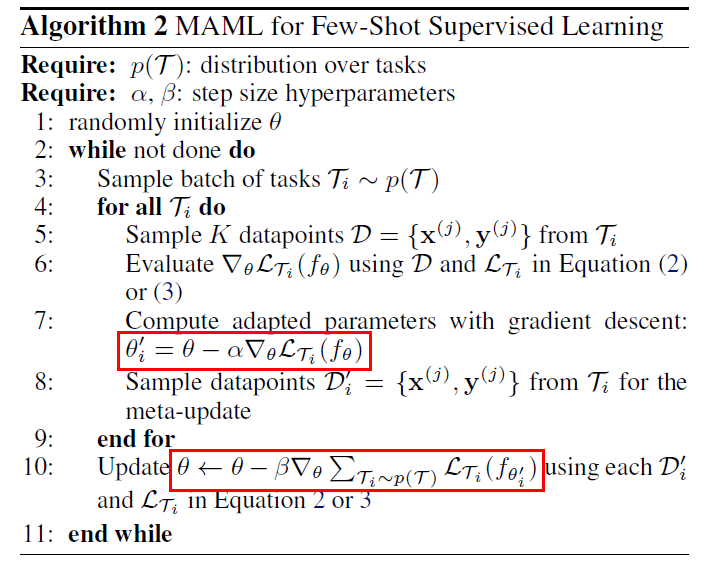
3-1. Supervised Regression & Classification
2개의 common loss function : MSE, cross entropy
(1) MSE
- \(\mathcal{L}_{\mathcal{T}_{i}}\left(f_{\phi}\right)=\sum_{\mathbf{x}^{(j)}, \mathbf{y}^{(j)} \sim \mathcal{T}_{i}}\left\|f_{\phi}\left(\mathbf{x}^{(j)}\right)-\mathbf{y}^{(j)}\right\|_{2}^{2}\).
(2) Cross Entropy
- \(\begin{aligned} \mathcal{L}_{\mathcal{T}_{i}}\left(f_{\phi}\right)=\sum_{\mathbf{x}^{(j)}, \mathbf{y}^{(j)} \sim \mathcal{T}_{i}} \mathbf{y}^{(j)} \log f_{\phi}\left(\mathbf{x}^{(j)}\right) &+\left(1-\mathbf{y}^{(j)}\right) \log \left(1-f_{\phi}\left(\mathbf{x}^{(j)}\right)\right) \end{aligned}\).
4. 기타
4-1. Multi-task vs Meta Learning
- Multi-task : task 별로 최적 parameter \(\phi_i\)가 모두 동일
- Meta : task 별로 최적 parameter \(\phi_i\)가 모두 다름
- \(D_{meta-train}\) 을 사용하여 “task 별 \(\phi_i\)들”을 학습하는게 아님!
- \(D_{meta-train}\) 을 사용하여 “데이터의 특성 & \(\phi_i\) 사이의 관계 정보 (=\(\theta\))” 를 학습!
- 새로운 데이터가 들어오면, 여기서 학습한 \(\theta\)를 사용하여 적은 데이터로도 빠르게 학습 가능!
4-2. Meta-Learning Approaches
대표적인 두 종류
- 1) Metric-based
- 2) Optimization-based
1) Metric based
-
1) \(D_{meta-train}\)을 사용하여 저차원에 embedding
2) 새로운 데이터가 들어오면, 이를 저차원에 embedding & 가장 가까운 class로 분류
-
example : Prototypical Networks for Few shot Learning
2) Optimization based
-
1) \(D_{meta-train}\)을 사용하여 “효율적인 update 방법에 관한 정보인 \(\theta\)“를 학습
2) 새로운 데이터가 들어오면, 빠르게 parameter를 adopt
-
example : MAML
Reference
- Model-Agnostic Meta-Learning for Fast Adaptation of Deep …
- http://dmqm.korea.ac.kr/activity/seminar/265