(paper) Graph Augmented Normalizing Flows for AD of MTS

Graph Augmented Normalizing Flows for AD of MTS (2022)

Contents

1. Abstract
2. Introduction
3. Preliminaries
   1. Normalizing Flows
   2. Bayesian Networks
4. Problem Statement
5. Method
   1. Factorization
   2. NN Parameterization
   3. Joint Training

0. Abstract

Anomaly Detection

• detecting anomalies for MTS is challenging… due to intricate interdependencies

• Hypothesize that “anomalies occur in LOW density regions of distn”

  \(\rightarrow\) use of NFs for unsupervised AD

GANF ( Graph Augmented NF )

propose a novel flow model, by imposing a Bayesian Network (BN)

• BN : DAG (Directed Acyclic Graph) that models causal relationships

  ( factorizes joint probability into product of easy-to-evaluate conditional probabilities )

1. Introduction

explore the use of NF for AD

• NF = DGM for learning underlying distn of data samples
• NF = unsupervised

Issue = “High dimensionality” & “Interdependency challenges”

\(\rightarrow\) solve by learning the relational structure among constituent series

Bayesian networks

• models “causal relationships”
• DAG, where node is “conditionally independent” of its non-descendents, given its parents
• allows factorizing the intractable joint density

GANF

• agument NF with “graph structure learning”
• apply to solve AD

2. Preliminaries

(1) Normalizing Flows

Notation

• MTS : \(\mathbf{x} \in \mathbb{R}^{D}\)
• NF : \(\mathbf{f}(\mathbf{x}): \mathbb{R}^{D} \rightarrow \mathbb{R}^{D}\)
  • normalizes the distribution of \(\mathbf{x}\) to a “standard” distribution ( base distribution )
• output of NF : \(\mathbf{z}=\mathbf{f}(\mathbf{x})\)
  • with pdf \(q(\mathbf{z})\)

Change of Variable :

density of the \(\mathbf{x}\), \(p(\mathbf{x})\) =

• \(\log p(\mathbf{x})=\log q(\mathbf{f}(\mathbf{x}))+\log \mid \operatorname{det} \nabla_{\mathbf{x}} \mathbf{f}(\mathbf{x}) \mid\).

Computaitonal Issues

• (1) Jacobian determinant needs to be easy to compute
• (2) \(f\) need to be invertible
  • \(\mathbf{x}=\mathbf{f}^{-1}(\mathbf{z})\).

ex) MAF (Masked Autoregressive Flow)

• output : \(\mathbf{z}=\left[z_{1}, \ldots, z_{D}\right]\).
• input : \(\mathbf{x}=\left[x_{1}, \ldots, x_{D}\right]\)
• mapping : \(z_{i}=\left(x_{i}-\mu_{i}\left(\mathbf{x}_{1: i-1}\right)\right) \exp \left(\alpha_{i}\left(\mathbf{x}_{1: i-1}\right)\right)\)
  • \(\mu_i\) & \(\alpha_i\) : NN

Conditional flow

• \(\mathbf{f}: \mathbb{R}^{D} \times \mathbb{R}^{d} \rightarrow \mathbb{R}^{D}\).

• Additional Info = flow may be augmented with conditional information \(\mathbf{h} \in \mathbb{R}^{d}\)

  ( may have different dimension )

• \(\log p(\mathbf{x} \mid \mathbf{h})=\log q(\mathbf{f}(\mathbf{x} ; \mathbf{h}))+\log \mid \operatorname{det} \nabla_{\mathbf{x}} \mathbf{f}(\mathbf{x} ; \mathbf{h}) \mid\).

NF for time series

• \(\mathbf{X}=\left[\mathbf{x}_{1}, \mathbf{x}_{2}, \ldots, \mathbf{x}_{T}\right]\), where \(\mathbf{x}_{t} \in \mathbb{R}^{D}\)

• via successive conditioning…

  • \(p(\mathbf{X})=p\left(\mathbf{x}_{1}\right) p\left(\mathbf{x}_{2} \mid \mathbf{x}_{<2}\right) \cdots p\left(\mathbf{x}_{T} \mid \mathbf{x}_{<T}\right)\).

  • Rasul et al. (2021) propose to model each \(p\left(\mathbf{x}_{t} \mid \mathbf{x}_{<t}\right)\) as \(p\left(\mathbf{x}_{t} \mid \mathbf{h}_{t-1}\right)\), where \(\mathbf{h}_{t-1}\) summarizes the \(\mathbf{x}_{<t}\)

(2) Bayesian Networks

Bayesian Network

= describes the conditional independence among variables

Notation

• \(X^{i}\) : general random variable
• \(n\) variables \(\left(X^{1}, \ldots, X^{n}\right)\) = nodes of DAG
• \(\mathbf{A}\) : weighted adjacency matrix
  • where \(\mathbf{A}_{i j} \neq 0\) if \(X^{j}\) is the parent of \(X^{i}\)

Density of the joint distribution of \(\left(X^{1}, \ldots, X^{n}\right)\) is

• \(p\left(X^{1}, \ldots, X^{n}\right)=\prod_{i=1}^{n} p\left(X^{i} \mid \operatorname{pa}\left(X^{i}\right)\right)\).

  where \(\operatorname{pa}\left(X^{i}\right)=\left\{X^{j}: \mathbf{A}_{i j} \neq 0\right\}\).

3. Problem Statement

Unsupervised Anomaly Detection with MTS

• training set \(\mathcal{D}\) : only UNlabeled data ( assume most of them are NOT anomalies )
• \(\mathcal{X} \in \mathcal{D}\) contains \(n\) constituent series with \(D\) attributes and of length \(T\)
  • \(\left(\mathbf{X}^{1}, \mathbf{X}^{2}, \ldots, \mathbf{X}^{n}\right)\), where \(\mathbf{X}^{i} \in \mathbb{R}^{T \times D}\).
• use a Bayesian network (DAG) to model the relational structure of the constituent series \(\mathbf{X}^{i}\)
• augment NF to compute density of \(\mathcal{X}\)
• \(\mathbf{A} \in \mathbb{R}^{n \times n}\) : adjacency matrix of DAG

Augmented Flow : \(\mathcal{F}:(\mathcal{X}, \mathbf{A}) \rightarrow \mathcal{Z}\)

• anomaly points : LOW densities
• conduct UNsupervised AD, by evaluating the density of a MTS computed through the augmented flow

4. Method

Graph Augmented NF : \(\mathcal{F}:(\mathcal{X}, \mathbf{A}) \rightarrow \mathcal{Z}\)

Central Idea : FACTORIZATION

• factorize \(p(\mathcal{X})\) along the…
  • (1) series dimension ( using Bayesian Network )
  • (2) temporal dimension ( using conditional NF )

(1) Factorization

Density of MTS \(\mathcal{X}=\left(\mathbf{X}^{1}, \mathbf{X}^{2}, \ldots, \mathbf{X}^{n}\right)\) :

• can be computed as the product of \(p\left(\mathbf{X}^{i} \mid \mathrm{pa}\left(\mathbf{X}^{i}\right)\right)\) for all nodes
• further factorize each conditional density along the temporal dimension

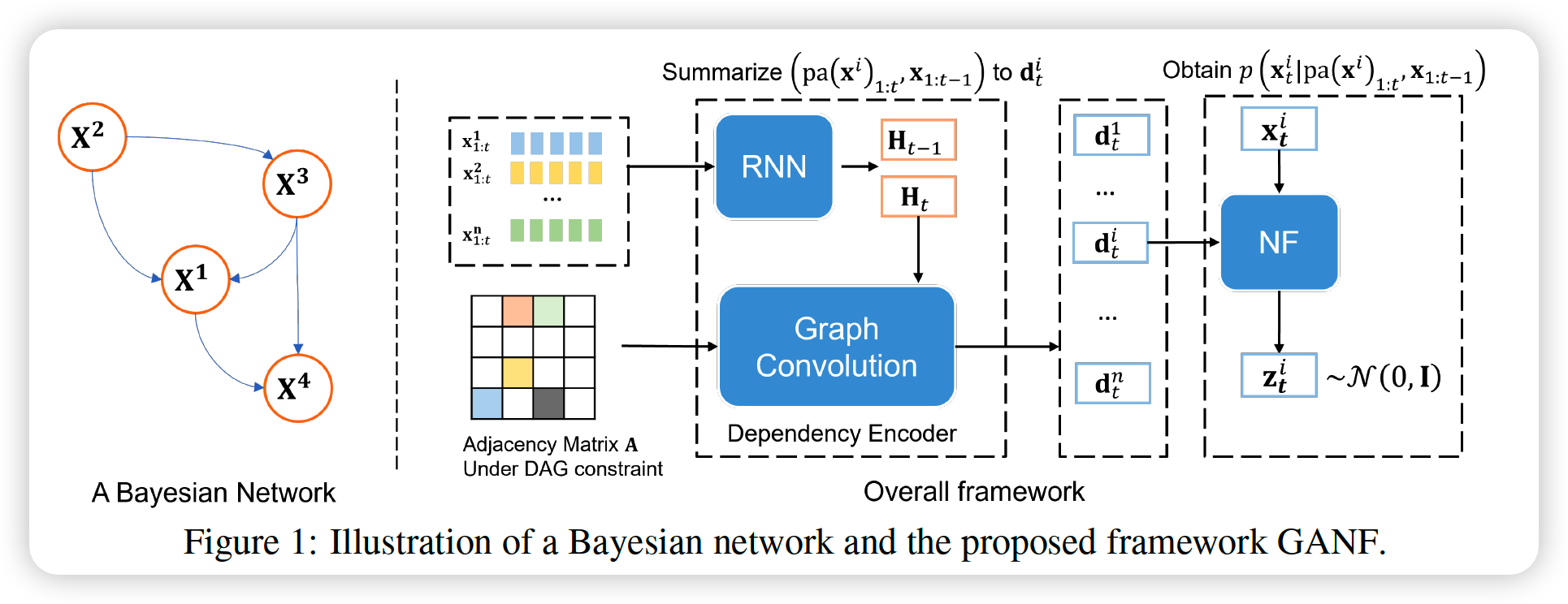
\(p(\mathcal{X})=\prod_{i=1}^{n} p\left(\mathbf{X}^{i} \mid \operatorname{pa}\left(\mathbf{X}^{i}\right)\right)=\prod_{i=1}^{n} \prod_{t=1}^{T} p\left(\mathbf{x}_{t}^{i} \mid \operatorname{pa}\left(\mathbf{x}^{i}\right)_{1: t}, \mathbf{x}_{1: t-1}^{i}\right)\).

• parameterize each conditional density \(p\left(\mathbf{x}_{t}^{i} \mid \operatorname{pa}\left(\mathbf{x}^{i}\right)_{1: t}, \mathbf{x}_{1: t-1}^{i}\right)\), by using a Graph-based dependency encoder

(2) NN Parameterization

conditional densities \(p\left(\mathbf{x}_{t}^{i} \mid \operatorname{pa}\left(\mathbf{x}^{i}\right)_{1: t}, \mathbf{x}_{1: t-1}^{i}\right)\)

• can be learned by using conditional NF

• Shape (Dimension Issue)

  • pa \(\left(\mathbf{x}^{i}\right)_{1: t}\) and \(\mathbf{x}_{1: t-1}^{i}\) cannot be directly used for parameterization!

  • thus, design a graph-based dependency encoder

    \(\rightarrow\) make it into \(d\)-dim fixed length vector

Dependency Encoder

step 1) use RNN to map MTS to fixed length vector

• \(\mathbf{h}_{t}^{i}=\operatorname{RNN}\left(\mathbf{x}_{t}^{i}, \mathbf{h}_{t-1}^{i}\right)\).
• Share RNN parameters across all nodes in DAG

step 2) GCN

• aggregate hidden states of the parents for dependency encoding

• output : \(\mathbf{D}_{t}=\left(\mathbf{d}_{t}^{1}, \ldots, \mathbf{d}_{t}^{n}\right)\), for all \(t\)

• \(\mathbf{D}_{t}=\operatorname{ReLU}\left(\mathbf{A H}_{t} \mathbf{W}_{1}+\mathbf{H}_{t-1} \mathbf{W}_{2}\right) \cdot \mathbf{W}_{3}\).

  • \(\mathbf{W}_{1} \in \mathbb{R}^{d \times d}\).
  • \(\mathbf{W}_{2} \in \mathbb{R}^{d \times d}\).
  • \(\mathbf{W}_{3} \in \mathbb{R}^{d \times d}\) ( additional transformation to improve performance )

Density Estimation

• with dependency encoder, obtain \(\mathbf{d}_{t}^{i}\)
• apply NF on \(\mathbf{d}_{t}^{i}\), to model each \(p\left(\mathbf{x}_{t}^{i} \mid \mathrm{pa}\left(\mathbf{x}^{i}\right)_{1: t}, \mathbf{x}_{1: t-1}^{i}\right)\)
  • NF : \(\mathbf{f}: \mathbb{R}^{D} \times \mathbb{R}^{d} \rightarrow \mathbb{R}^{D}\)
• parameters of NF are also shared!
• conditional density of \(x_t^{i}\) :
  • \(\log p\left(\mathbf{x}_{t}^{i} \mid \operatorname{pa}\left(\mathbf{x}^{i}\right)_{1: t}, \mathbf{x}_{1: t-1}^{i}\right)=\log p\left(\mathbf{x}_{t}^{i} \mid \mathbf{d}_{t}^{i}\right)=\log q\left(\mathbf{f}\left(\mathbf{x}_{t}^{i} ; \mathbf{d}_{t}^{i}\right)\right)+\log \mid \operatorname{det} \nabla_{\mathbf{x}_{t}^{i}} \mathbf{f}\left(\mathbf{x}_{t}^{i} ; \mathbf{d}_{t}^{i}\right) \mid\).
• example of \(f\) : RealNVP, MAF …

Log Density of MTS

• \(\log p(\mathcal{X})=\sum_{i=1}^{n} \sum_{t=1}^{T}\left[\log q\left(\mathbf{f}\left(\mathbf{x}_{t}^{i} ; \mathbf{d}_{t}^{i}\right)\right)+\log \mid \operatorname{det} \nabla_{\mathbf{x}_{t}^{\mathbf{f}}} \mathbf{f}\left(\mathbf{x}_{t}^{i} ; \mathbf{d}_{t}^{i}\right) \mid \right]\).

Anomaly Measures

• use the density computed by \(\log p(\mathcal{X})\)

  • lower density = more likely anomaly

• also produces conditional densities for each constituent series

  • conditional densities : \(\log p\left(\mathbf{X}^{i} \mid \mathrm{pa}\left(\mathbf{X}^{i}\right)\right)=\) \(\sum_{t=1}^{T} \log p\left(\mathbf{x}_{t}^{i} \mid \mathbf{d}_{t}^{i}\right)\)
  • use this as anomaly measure

  ( low density \(p(\mathcal{X})\) is caused by one or a few low conditional densities \(p\left(\mathbf{X}^{i} \mid \mathrm{pa}\left(\mathbf{X}^{i}\right)\right)\) )

(3) Joint Training

Training Objective

= joint density (likelihood) of the observed data

= KL-divergence between true distn & recovered distn

(with DAG constraint…)

\(\min _{\mathbf{A}, \boldsymbol{\theta}} \mathcal{L}(\mathbf{A}, \boldsymbol{\theta})=\frac{1}{ \mid \mathcal{D} \mid } \sum_{i=1}^{ \mid \mathcal{D} \mid }-\log p\left(\mathcal{X}_{i}\right)\).

s.t. \(h(\mathbf{A})=\operatorname{tr}\left(e^{\mathbf{A} \circ \mathbf{A}}\right)-n=0\)