(paper) SSL11 - Label Propagation

Label Propagation for Deep Semi-supervised Learning (2019)

Contents

1. Abstract
2. Preliminaries
3. Method
   1. Overview
   2. Nearest Neighbor Graph
   3. Label Propagation
   4. Pseudo-label certainty & Class balancing

0. Abstract

Classic methods on SSL

• focused on transductive learning

transductive label propagation method, based on the manifold assumption

• step 1) make predictions on the entire dataset
• step 2) use these predictions to generate pseudo-labels for the unlabeled data
• step 3) train a deep neural network

1. Preliminaries

(1) Problem Formulation

• \(n\) examples : \(X:=\left(x_1, \ldots, x_l, x_{l+1}, \ldots, x_n\right)\)

  • \(x_i \in \mathcal{X}\).

  • (1) first \(l\) examples :

    • input : \(X_L\) ….. \(x_i\) for \(i \in L:=\{1, \ldots, l\}\)

    • label : \(Y_L:=\left(y_1, \ldots, y_l\right)\) with \(y_i \in C\), where \(C:=\{1, \ldots, c\}\)

  • (2) remaining \(u:=n-l\) examples :

    • input : \(X_U\) … for \(i \in U:=\{l+1, \ldots, n\}\)
    • unlabeled

• goal of SSL :

  • use all examples \(X\) and labels \(Y_L\) to train a classifier

(2) Classifier

Model ( Classifier ) : \(f_\theta: \mathcal{X} \rightarrow \mathbb{R}^c\)

Divided in two parts

• (1) feature extraction network \(\phi_\theta: \mathcal{X} \rightarrow \mathbb{R}^d\)
  • embedding ( = descriptor ) : \(\mathbf{v}_i:=\phi_\theta\left(x_i\right)\)
• (2) fully connected (FC) layer applied on top of \(\phi_\theta\) + softmax
  • produce a vector of confidence scores

Output of the Classifier : \(f_\theta\left(x_i\right)\)

• predicted class : \(\hat{y}_i:=\arg \max _j f_\theta\left(x_i\right)_j\)

(3) Supervised Loss

\(L_s\left(X_L, Y_L ; \theta\right):=\sum_{i=1}^l \ell_s\left(f_\theta\left(x_i\right), y_i\right)\).

• only for labeled examples in \(X_L\)
• standard choice : (classification) CE loss
  • \(\ell_s(\mathbf{s}, y):=-\log \mathbf{s}_y\), for \(\mathbf{s} \in \mathbb{R}^c\) and \(y \in C\)

(4) Pseudo-Labeling

process of assigning a pseudo-label \(\hat{y}_i\) to each example \(x_i\) for \(i \in U\)

• notation : \(\hat{Y}_U:=\) \(\left(\hat{y}_{l+1}, \ldots, \hat{y}_n\right)\)

Pseudo-label loss term : \(L_p\left(X_U, \hat{Y}_U ; \theta\right):=\sum_{i=l+1}^n \ell_s\left(f_\theta\left(x_i\right), \hat{y}_i\right)\)

(5) Unsupervised Loss

Consistency Loss

• applied to both labeled and unlabeled examples

• encourages consistency under different transformations of the data

Loss function : \(L_u(X ; \theta):=\sum_{i=1}^n \ell_u\left(f_\theta\left(x_i\right), f_{\tilde{\theta}}\left(\tilde{x}_i\right)\right)\).

• \(\tilde{x}_i\) : different transformation of example \(x_i\)
• ex) \(\left.\ell_u(\mathbf{s}, \tilde{\mathbf{s}}):=\mid \mid \mathbf{s}-\tilde{\mathbf{s}}\right) \mid \mid ^2\).

(6) Transductive Learning

( Instead of training a generic classifier able to classify new data …. )

Goal : use \(X\) & \(Y_L\) to infer labels for examples in \(X_U\)

\(\rightarrow\) this paper : adopt graph based approach for transductive learning by diffusion

(7) Diffusion for Transductive Learning

Notation

• descriptor set : \(\left(\mathbf{v}_1, \ldots, \mathbf{v}_l, \mathbf{v}_{l+1}, \ldots, \mathbf{v}_n\right)\)
• symmetric adjacency matrix : \(W \in \mathbb{R}^{n \times n}\)
  • zero-diagonal
  • \(w_{i j}\) : non-neg pairwise similiarity
• symmetrically normalized version : \(\mathcal{W}=D^{-1 / 2} W D^{-1 / 2}\)
  • degree matrix : \(D:=\operatorname{diag}\left(W \mathbf{1}_n\right)\)
• \(n \times c\) label matrix : \(Y\)
  • \(Y_{i j}:= \begin{cases}1, & \text { if } i \in L \wedge y_i=j \\ 0, & \text { otherwise. }\end{cases}\).

Diffusion : \(Z:=(I-\alpha \mathcal{W})^{-1} Y\)

• where \(\alpha \in[0,1)\) is a parameter

Class prediction with diffusion : \(\hat{y}_i:=\arg \max _j z_{i j}\)

• where \(z_{i j}\) is the \((i, j)\) element of matrix \(Z\).

2. Method

(1) Overview

introduce a new iterative process for SSL

• step 1) construct a neareset neighbor graph
• step 2) perform label propagation for unlabeled data
• step 3) inject the obtained labels into network training process

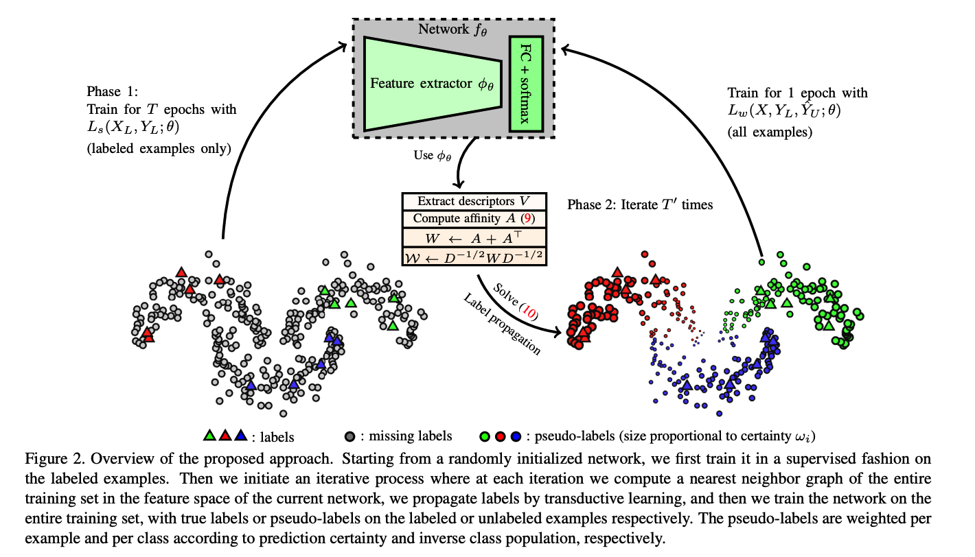
(2) Nearest Neighbor Graph

descriptor set \(V=\) \(\left(\mathbf{v}_1, \ldots, \mathbf{v}_l, \mathbf{v}_{l+1}, \ldots, \mathbf{v}_n\right)\)

• where \(\mathbf{v}_i:=\phi_\theta\left(x_i\right)\)

sparse affinity matrix \(A \in \mathbb{R}^{n \times n}\)

• where \(a_{i j}:= \begin{cases}{\left[\mathbf{v}_i^{\top} \mathbf{v}_j\right]_{+}^\gamma,} & \text { if } i \neq j \wedge \mathbf{v}_i \in \mathbf{N N}_k\left(\mathbf{v}_j\right) \\ 0, & \text { otherwise }\end{cases}\).

affinity matrix of the nearest neighbor graph is efficient even for large \(n\)

\(\leftrightarrow\) full affinity matrix : not tractable

let \(W:=A+A^{\top}\).

\(\rightarrow\) symmetric nonnegative adjacency matrix with zero diagonal.

(3) Label Propagation

Estimating matrix \(Z\) by \(Z:=(I-\alpha \mathcal{W})^{-1} Y\) is impractical for large \(n\)

\(\because\) \((I-\alpha \mathcal{W})^{-1}\) is not spares

Instead, use conjugate gradient (CG) method to solve ..

• \((I-\alpha \mathcal{W}) Z=Y\).
• faster than the iterative solution

With above … infer pseudo labels \(\hat{Y}_U=\left(\hat{y}_{l+1}, \ldots, \hat{y}_n\right)\).

• via \(\hat{y}_i:=\arg \max _j z_{i j}\).

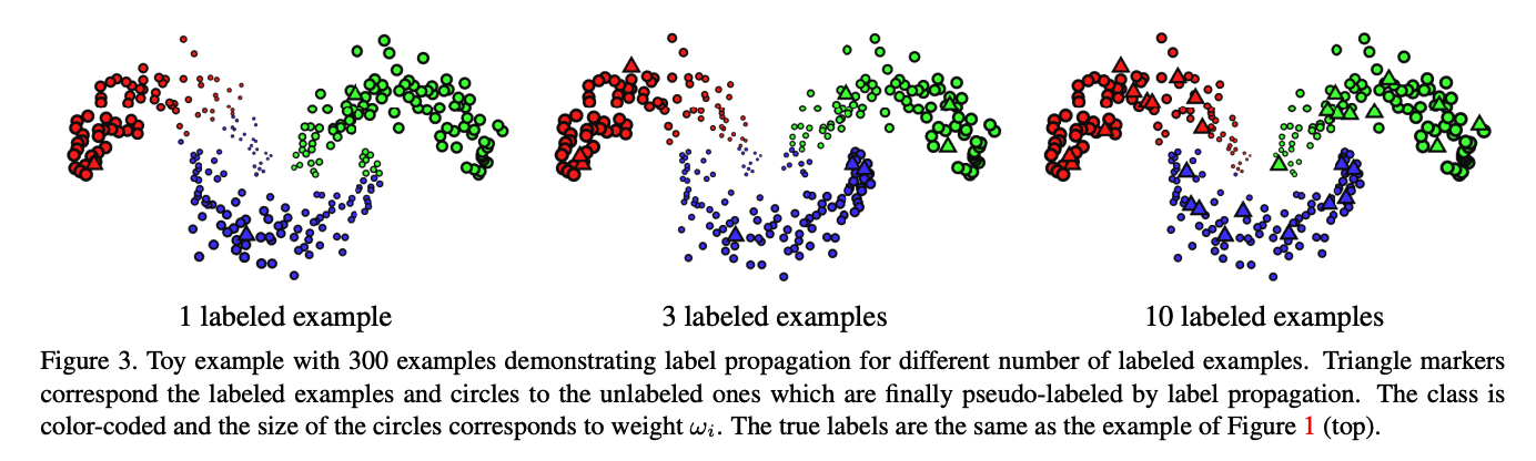
(4) Pseudo-label certainty & Class balancing

Inferring pseudo-labels from matrix \(Z\) by hard assignment

\(\rightarrow\) has two undesired effects

(1) cannot consider uncertainty

• do not have the same certainty for each data

(2) pseudo-labels may not be balanced over classes

• may impede learning

Solution to (1) …. per-example weight

use weight to reflect the certainty of the prediction

• use entropy as a measure

• weight : \(\omega_i:=1-\frac{H\left(\hat{\mathbf{z}}_i\right)}{\log (c)}\).

  • \(\hat{Z}\) : row-wise normalized version of \(Z\)

    ( \(\hat{z}_{i j}=z_{i j} / \sum_k z_{i k}\) )

  • \(H: \mathbb{R}^c \rightarrow \mathbb{R}\) : entropy function

  • \(\log (c)\) : maximum possible entropy

Solution to (2) …. per-class weight

assign weight \(\zeta_j\) to class \(j\)

• inversely proportional to class population
• \(\zeta_j:=\left( \mid L_j \mid + \mid U_j \mid \right)^{-1}\).

Weighted Loss

\(\begin{aligned} L_w\left(X, Y_L, \hat{Y}_U ; \theta\right) &:=\sum_{i=1}^l \zeta_{y_i} \ell_s\left(f_\theta\left(x_i\right), y_i\right) +\sum_{i=l+1}^n \omega_i \zeta_{\hat{y}_i} \ell_s\left(f_\theta\left(x_i\right), \hat{y}_i\right) \end{aligned}\).

• \(L_s\left(X_L, Y_L ; \theta\right):=\sum_{i=1}^l \ell_s\left(f_\theta\left(x_i\right), y_i\right)\)…. supervised loss
• \(L_p\left(X_U, \hat{Y}_U ; \theta\right):=\sum_{i=l+1}^n \ell_s\left(f_\theta\left(x_i\right), \hat{y}_i\right)\)…. pseudo-label loss