(paper) SSL12(1) - An Overview of Deep Semi-Supervised Learning (Consistency Regularization)

An Overview of Deep Semi-Supervised Learning (2020) - Part 1

Contents

1. Abstract
2. Introduction
   1. SSL
   2. SSL Methods
   3. Main Assumptions in SSL
   4. Related Problems
3. Consistency Regularization
   1. Ladder Networks
   2. Pi-Model
   3. Temporal Ensembling
   4. Mean Teachers
   5. Dual Students
   6. Fast-SWA
   7. Virtual Adversarial Training (VAT)
   8. Adversarial Dropout (AdD)
   9. Interpolation Consistency Training (ICT)
   10. Unsupervised Data Augmentation
4. Entropy Minimization
5. Proxy-label Methods
   1. Self-training
   2. Multi-view Training
6. Holistic Methods
   1. MixMatch
   2. ReMixMatch
   3. FixMatch
7. Generative Models
   1. VAE for SSL
   2. GAN for SSL
8. Graph-Based SSL
   1. Graph Construction
   2. Label Propagation
9. Self-Supervision for SSL

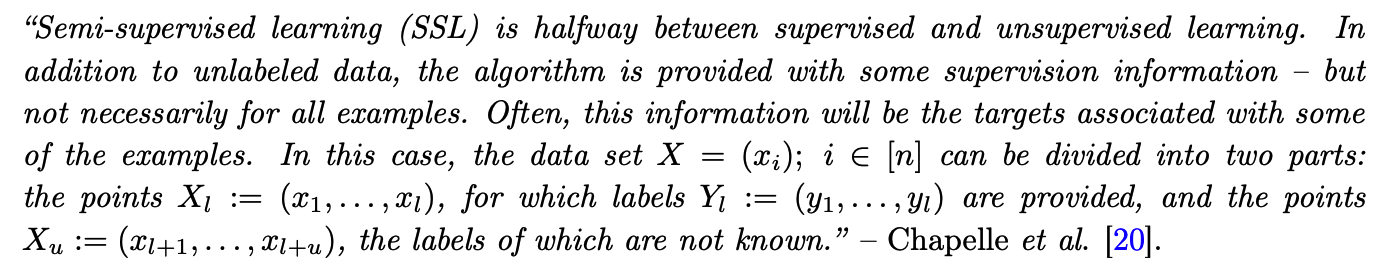
0. Abstract

semi-supervised learning (SSL)

• overcome the need for large annotated datasets

This paper :

\(\rightarrow\) provide a comprehensive overview of Deep SSL

1. Introduction

(1) SSL

(2) SSL Methods

can be divided into following categories

1. Consistency Regularization

   • small perturbation in input … small change in output

2. Proxy-label Methods

   • produce additional training examples

3. Generative Models

   • learned features on one task can be transferred to other downstream tasks

   • Generative models that generate images from \(p(x)\) ,

     must learn transferable features to a supervised task \(p(y \mid x)\)

4. Graph-based Methods

5. Entropy Minimization

   • force to make confident predictions

based on 2 dominant learning paradigims

• (1) transductive learning
  • apply the trained classifier on the unlabeled instances observed at training time
  • does not generalize to unobserved instances
  • mainly used on graphs
• (2) inductive learning
  • more popular paradigm
  • capable of generalizing to unobserved instances at test time

(3) Main Assumptions in SSL

( refer to https://seunghan96.github.io/ssl/SemiSL_intro/ )

(4) Related Problems

a) Active Learning

• provided with a large pool of unlabeled data

• aims to carefully choose the examples to be labeled to achieve a higher accuracy
• [ domain ] where data may be abundant, but labels are scarce

2 widely used selection criteria

• (1) informativeness
  • how well an unlabeled instance helps reduce the uncertainty of a statistical model
• (2) representativeness
  • how well an instance helps represent the structure of input patterns

Active Learning & SSL : both aim to use a limited amount of data to improve model

b) Transfer Learning & Domain Adaptation

Transfer learning (TL) :

• to improve a learner on target domain, by transferring the knowledge learned from source domain
• ex) Domain Adaptation (DA)

Domain Adaptation (DA)

• Goal : train a learner capable of generalizing across different domains of different distributions,

  where..

  • (1) much labeled data for source domain

  • (2) no/less/fully labeled data for target domain - no : unsupervised DA - less : semi-supervised DA - fully : supervised DA

SSL & unsupervised DA

• (common)
  • provided with labeled and unlabeled data
  • goal : learning a function capable of generalizing to the unlabeled/unseen data
• (difference)
  • SSL : both labeled & unlabeld come from SAME distn
  • unsupervised DA : both labeled & unlabeld come from DIFFERENT distn

c) Weakly-supervised Learning

Goal : same as supervised learning

Difference : instead of GT label … provided with weakly annotated examples

• ex) crowd workers, output of other classifiers….

Example )

• weakly-supervised semantic segmentation,
  • pixel-level labels are substituted for inexact annotations

\(\rightarrow\) SSL can be used to enhance the performance

d) Learning with Noisy labels

If the noise is significant….. can harm much!

\(\rightarrow\) to overcome this, s seek to correct the loss function!

Type of correction :

• [ex 1] SAME weight for all samples
  • relabel the noisy examples ( where proxy labels methods can be used )
• [ex 2] DIFFERENT ~
  • reweighing to the training examples to distinguish between the clean and noisy

SSL & Noisy Labels

• noisy examples are considered as unlabeled data

  & used to regularize training using SSL methods

2. Consistency Regularization

Trend in Deep SSL :

• use the unlabeled data to enforce the trained model to be in line with the cluster assumption

  ( = the learned decision boundary must lie in low-density regions )

\(\rightarrow\) if small perturbation …. prediction should not change significantly

Favor functions \(f_\theta\) that give consistent predictions for similar data points.

• pushing the decision boundaries away from the unlabeled data points

Mathematical Expression

• given \(x \in \mathcal{D}_u\) & perturbed version \(\hat{x}_u\)
• Goal : minimize \(d\left(f_\theta(x), f_\theta(\hat{x})\right)\)
  • ex) MSE, KL-div, JS-div
• \(f_\theta(x)\) & \(f_\theta(\hat{x})\) : form of pdf over \(C\) classes
  • let \(m=\frac{1}{2}\left(f_\theta(x)+f_\theta(\hat{x})\right)\)

Various distance metrics :

• \(d_{\mathrm{MSE}}\left(f_\theta(x), f_\theta(\hat{x})\right)=\frac{1}{C} \sum_{k=1}^C\left(f_\theta(x)_k-f_\theta(\hat{x})_k\right)^2\).
• \(d_{\mathrm{KL}}\left(f_\theta(x), f_\theta(\hat{x})\right)=\frac{1}{C} \sum_{k=1}^C f_\theta(x)_k \log \frac{f_\theta(x)_k}{f_\theta(\hat{x})_k}\).
• \(d_{\mathrm{JS}}\left(f_\theta(x), f_\theta(\hat{x})\right)=\frac{1}{2} d_{\mathrm{KL}}\left(f_\theta(x), m\right)+\frac{1}{2} d_{\mathrm{KL}}\left(f_\theta(\hat{x}), m\right)\).

( can also enforce a consistency over two perturbed versions of \(x, \hat{x}_1\) and \(\hat{x}_2\). )

(1) Ladder Networks

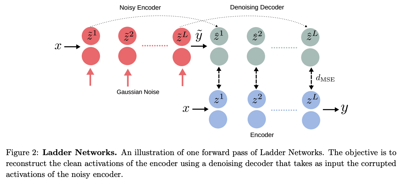
Ladder Networks, with an additional encoder and decoder for SSL

• Consists of 2 encoders & 1 decoder
  • encoder # 1 : corrupted
  • encoder # 2 : clean

a) Process

• input \(x\) is passed through 2 encoders
  • corrupted encoder : Gaussian noise is injected at each layer
    • output 1 : corrupted prediction \(\tilde{y}\)
  • clean encoder :
    • output 2 : clean prediction \(y\)
• \(\tilde{y}\) is fed into decoder
  • Reconstruct the uncorrupted input \(x\) & clean hidden activations \(z\)
• unsupervised loss ( \(\mathcal{L}_u\) ) : MSE between \(z\) & \(\tilde{z}\)

( computed over all layers, with a weighting \(\lambda_l\) )

b) Loss Functions

Unsupervised loss ( \(\mathcal{L}_u\) )

• \(\mathcal{L}_u=\frac{1}{ \mid \mathcal{D} \mid } \sum_{x \in \mathcal{D}} \sum_{l=0}^L \lambda_l d_{\mathrm{MSE}}\left(z^{(l)}, \hat{z}^{(l)}\right)\).

Supervised loss

• CE loss ( \(\mathrm{H}(\tilde{y}, t)\) )

Final Loss

• \(\mathcal{L}=\mathcal{L}_u+\mathcal{L}_s=\mathcal{L}_u+\frac{1}{ \mid \mathcal{D}_l \mid } \sum_{x, t \in \mathcal{D}_l} \mathrm{H}(\tilde{y}, t)\).

Summary

• can be easily adapted for CNN

• BUT …. computationally heavy

  \(\rightarrow\) to mitigate this …. propose variant of ladder networks , called \(\Gamma-\)model

• \(\Gamma-\)model

  • \(\lambda_l=0\) when \(l<L\)
  • decoder is omitted
  • unsupervised loss is computed as MSE between \(y\) & \(\tilde{y}\)

(2) Pi (\(\Pi\)) -Model

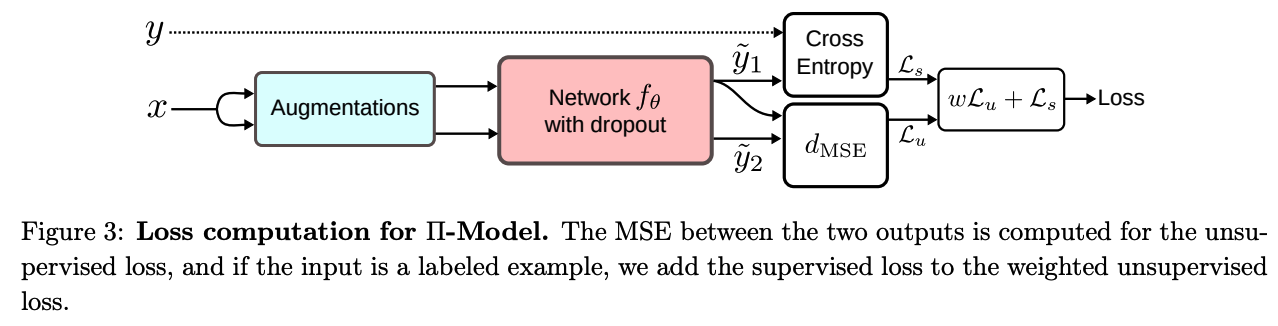
• simplification of the \(\Gamma\)-Model of Ladder Networks

Modifications

• corrupted encoder is removed

  ( just use the same network to get corrupted & uncorrupted inputs )

• takes advantage of the stochastic nature of the prediction function \(f_\theta\)

  • due to common regularization techniques ( such as DA, dropout …. )

• objectives

  • (1) reduce the distances between two predictions of \(f_\theta\) ( = \(d(y, \tilde{y}))\)
  • (2) obtain consistent predictions for both

Loss function

• \(\mathcal{L}=w \frac{1}{ \mid \mathcal{D}_u \mid } \sum_{x \in \mathcal{D}_u} d_{\mathrm{MSE}}\left(\tilde{y}_1, \tilde{y}_2\right)+\frac{1}{ \mid \mathcal{D}_l \mid } \sum_{x, y \in \mathcal{D}_l} \mathrm{H}(y, f(x))\).

• \(w\) : weighting function

  • starting from 0 up to a fixed weight \(\lambda(e . g ., 30)\)

  \(\rightarrow\) avoid using the untrained and random prediction function

(3) Temporal Ensembling

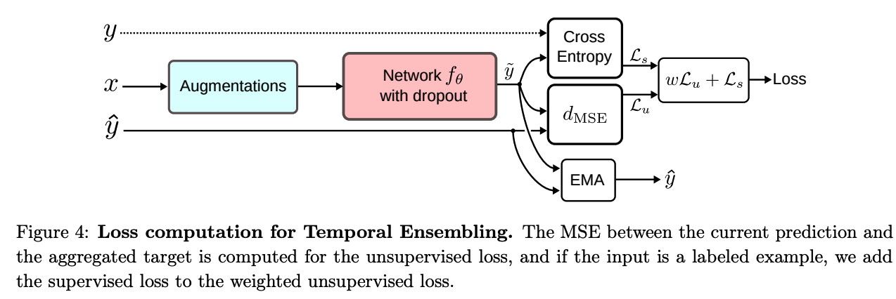
Divided into two stages

• step 1) classify all of the training data
  • without updating the weights
  • obtain \(y\)
• step 2) consider \(y\) as targets for unsupervised loss
  • to enforce consistency of predictions
  • minimize distance between “current output \(\tilde{y}\) ” and “\(y\)”
    • obtain \(\tilde{y}\) under different dropouts and augmentations

Problem ?

• target \(y\) is based on single evaluation & change over time…. instability!

\(\rightarrow\) propose Temporal Ensembling ( 2nd version of \(\Pi\) -model )

Temporal Ensembling :

• target \(y_{\text{ema}}\) is the “aggregation of all previous predictions”
  • \(y_{\mathrm{ema}}=\alpha y_{\mathrm{ema}}+(1-\alpha) \tilde{y}\).
• result : speed up the training time 2 x

At the start of training ….. Temporal Ensembling \(\approx\) \(\Pi\)-model

\(\because\) aggregated targets are very noisy!

\(\rightarrow\) ( like bias correction in Adam optimizer …. )

• \(y_{\mathrm{ema}}=\left(\alpha y_{\mathrm{ema}}+(1-\alpha) \tilde{y}\right) /\left(1-\alpha^t\right)\).

(4) Mean Teachers

\(\Pi\)-model & Temporal Ensembling :

• better & more stable teacher model ( by using EMA of predictions )

• ensembling : improves performance…

  BUT problem?

  • (1) newly learned information is incorporated slowly!

  • (2) same model plays a dual role ( student & teacher )

Solution : quality of the targets must be improved

• (1) carefully choosing the perturbations ( instead of just adding noise )
• (2) carefully choosing the teacher model ( instead of copying student model )

\(\rightarrow\) propose Mean Teacher

Mean Teacher

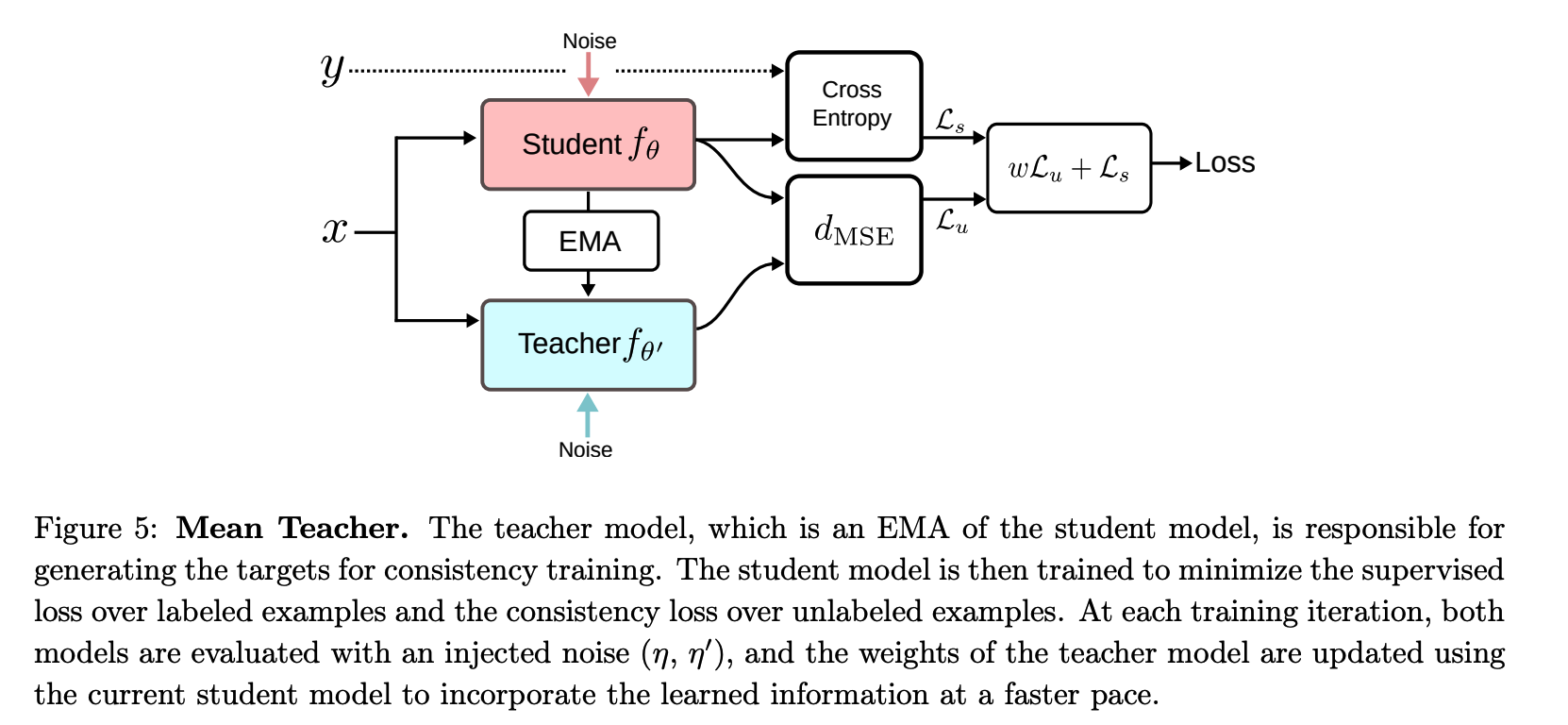
• proposes using a teacher model for a faster incorporation of the learned signal

Difference with other models :

• [ \(\Pi\)-Model ] : uses the same model as a student and a teacher \(\theta^{\prime}=\theta\)
• [ Temporal Ensembling ] : approximate a stable teacher \(f_{\theta^{\prime}}\) as an ensemble function with a weighted average of successive predictions
• [ Mean Teacher ] : defines the weights \(\theta_t^{\prime}\) of the teacher model \(f_{\theta^{\prime}}\) at a training step \(t\) as an EMA of successive student’s weights \(\theta\) :
  • \(\theta_t^{\prime}=\alpha \theta_{t-1}^{\prime}+(1-\alpha) \theta_t\).

Loss Function :

\(\mathcal{L}=w \frac{1}{ \mid \mathcal{D}_u \mid } \sum_{x \in \mathcal{D}_u} d_{\mathrm{MSE}}\left(f_\theta(x), f_{\theta^{\prime}}(x)\right)+\frac{1}{ \mid \mathcal{D}_l \mid } \sum_{x, y \in \mathcal{D}_l} \mathrm{H}\left(y, f_\theta(x)\right)\).

(5) Dual Students

main drawbacks of using a Mean Teacher :

\(\rightarrow\) given a large number of training iterations, the teacher model weights will converge to that of the student model

• biased & unstable predictions will be carried over to the student

Solution : Dual Students ( \(f_{\theta_1}\) and \(f_{\theta_2}\) )

• 2 student models with different initialization

  • one of them provides the targets for the other
    • which one? test for more stable predictions

• stability conditions :

  • (1) \(f(x)=f(\tilde{x})\)

  • (2) \(f(x)\) is greater than a confidence threshold \(\epsilon\)

    ( = far from decision boundary )

Compute 4 predictions

• \(f_{\theta_1}(x), f_{\theta_1}(\tilde{x}), f_{\theta_2}(x)\), and \(f_{\theta_2}(\tilde{x})\)

Loss Function

\(\begin{aligned}\mathcal{L}&=\mathcal{L}_s+\lambda_1 \mathcal{L}_u\\&=\frac{1}{ \mid \mathcal{D}_l \mid } \sum_{x, y \in \mathcal{D}_l} \mathrm{H}\left(y, f_{\theta_i}(x)\right)+\lambda_1 \frac{1}{ \mid \mathcal{D}_u \mid } \sum_{x \in \mathcal{D}_u} d_{\mathrm{MSE}}\left(f_{\theta_i}(x), f_{\theta_i}(\tilde{x})\right)\end{aligned}\).

[ + \(\alpha\) ] force one of the students to have similar predictions to its counterpart

which one to update its weights ?

\(\rightarrow\) check for both models’ stability constraint

• if unstable model … update that model!
• if both stable …. update the model with the largest variation \(\mathcal{E}^i= \mid \mid f_i(x)-f_i(\tilde{x}) \mid \mid ^2\)

The least stable model is trained with an additional loss:

• \(\lambda_2 \sum_{x \in \mathcal{D}_u} d_{\mathrm{MSE}}\left(f_{\theta_i}(x), f_{\theta_j}(x)\right)\).

(6) Fast-SWA

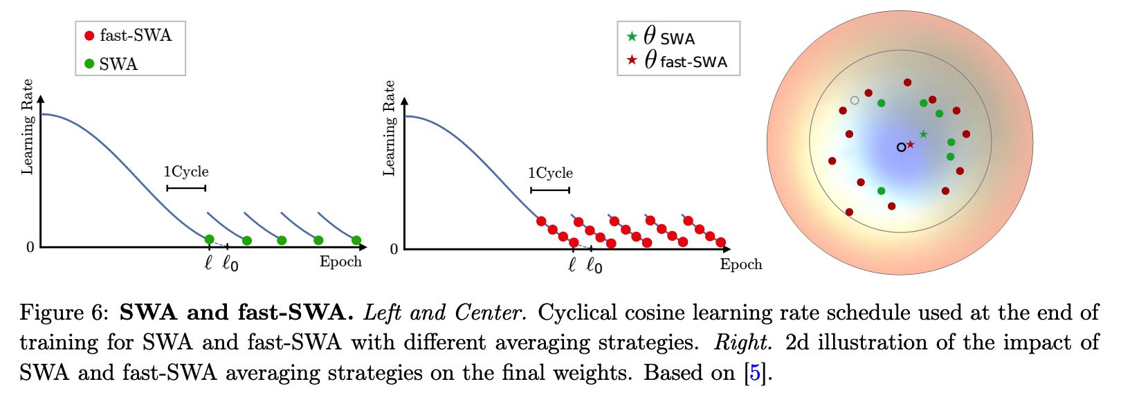
Findings :

• \(\Pi\)-Model & Mean Teacher : continue taking significant steps in the weight space at the end of training

• averaging the SGD iterates can lead to final weights closer to the center of the flat region

  ( thus stabilizing the SGD trajectory )

Ensemble of the model LATE in training :

• Stochastic Weight Averaging (SWA)
  • approach based on averaging the weights traversed by SGD at the end of training with a cyclic learning rate

• Fast-SWA

  • modifictiaon of SWA

  • averages the networks to many points during the same cycle

    ( resulting in better final model & faster ensembling procedure )

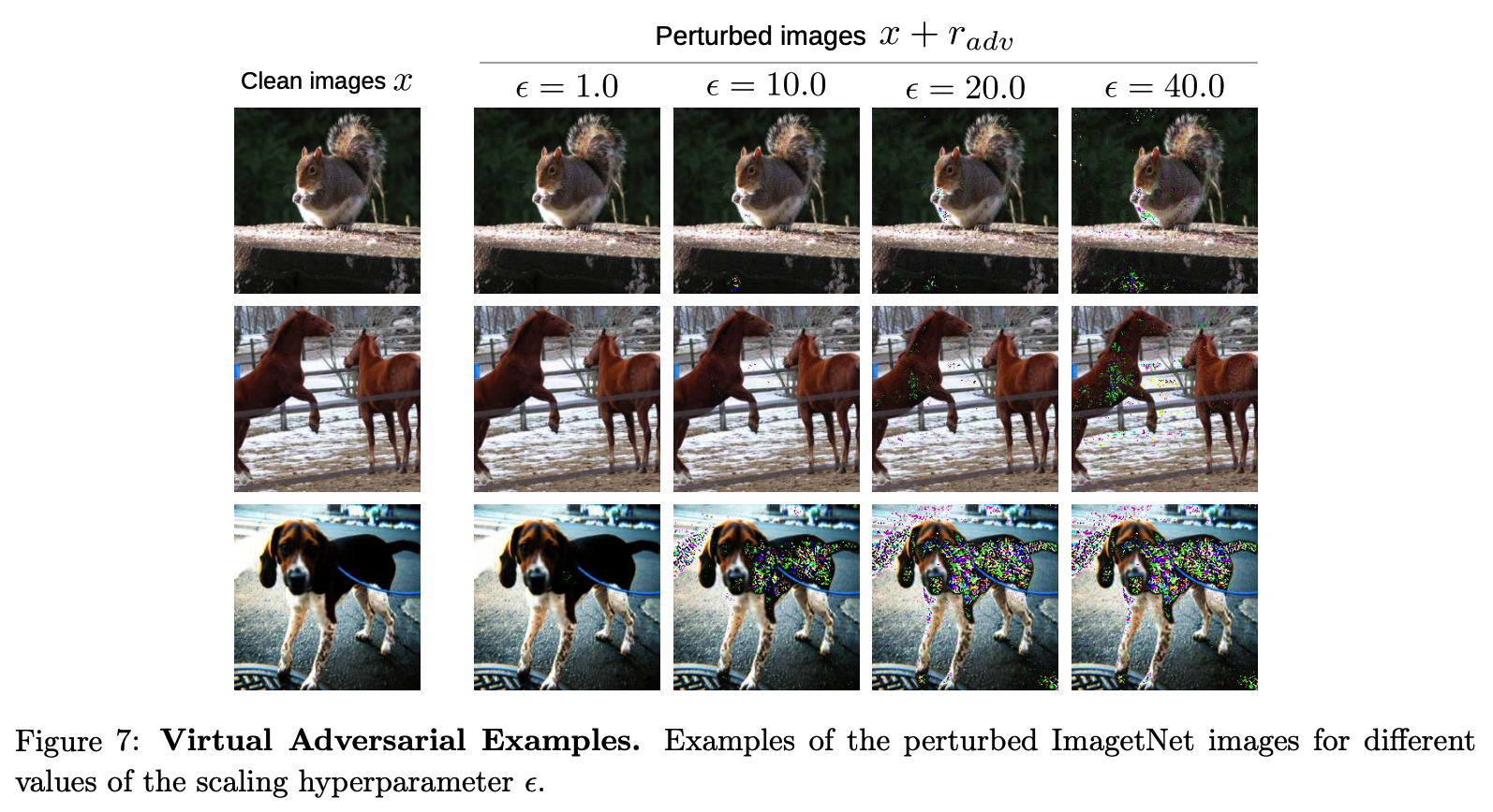
(7) Virtual Adversarial Training (VAT)

Previous approaches :

• applying random perturbations to each input

  & encouraging the model to assign similar outputs

\(\rightarrow\) push for a smoother output distribution

HOWEVER, random noise and random data augmentation…

\(\rightarrow\) leaves the predictor vulnerable to small perturbations in a specific direction ( = adversarial direction )

Adversarial Direction

• direction in the input space in which the label probability \(p(y \mid x)\) of the model is most sensitive

Virtual Adversarial Training (VAT)

( inspired by adversarial training )

• trains the model to assign to each input data a label that is similar to the labels of its neighbors in the adversarial direction
• a regularization technique that enhances the model’s robustness around each input data point against random and local perturbations
• Why Virtual ?
  • adversarial perturbation is approximated without any label information

[ Procedure ]

1. \[r \sim \mathcal{N}\left(0, \frac{\xi}{\sqrt{\operatorname{dim}(x)}} I\right)\]
2. \[\operatorname{grad}_r=\nabla_r d_{\mathrm{KL}}\left(f_\theta(x), f_\theta(x+r)\right)\]
3. \[r_{a d v}=\epsilon \frac{\operatorname{grad}_r}{ \mid \mid \operatorname{grad_{r} \mid \mid }}\]

Loss Function

\(\mathcal{L}_u=w \frac{1}{ \mid \mathcal{D}_u \mid } \sum_{x \in \mathcal{D}_u} d_{\mathrm{MSE}}\left(f_\theta(x), f_\theta\left(x+r_{a d v}\right)\right)\).

Additional

• For a more stable training, a Mean Teacher can be used to generate stable targets!

  \(\rightarrow\) by replacing \(f_\theta(x)\) with \(f_{\theta^{\prime}}(x)\) ( where \(f_{\theta^{\prime}}\) is an EMA of the student \(f_\theta\) )

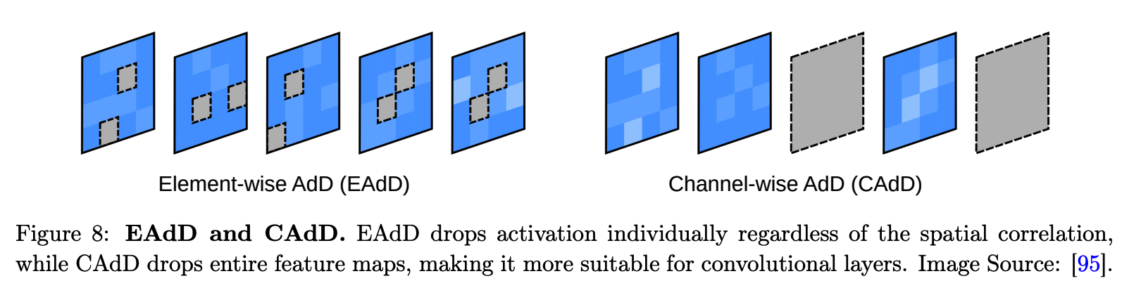
(8) Adversarial Dropout (AdD)

( Instead of using an additive adversarial noise as VAT )

a) element-wise adversarial dropout (EAdD)

• dropout masks are adversarially optimized to alter the model’s predictions
• induce a sparse structure of the neural network

Find the dropout conditions that are most sensitive to the model’s predictions.

• do not have access to the true labels

  ( instead, use the model’s predictions on the unlabeled data points to approximate the adversarial dropout mask \(\epsilon^{a d v}\) ….. where \(\mid \mid \epsilon^{a d v}-\epsilon \mid \mid _2 \leq \delta H)\)

Start with random dropout mask & update it in an adversarial manner

Notation :

• prediction function \(f_\theta\)
  • divided into \(f_\theta(x, \epsilon)=f_{\theta_2}\left(f_{\theta_1}(x) \odot \epsilon\right)\)
• approximation of Jacobian matrix :
  • \(J(x, \epsilon) \approx f_{\theta_1}(x) \odot \nabla_{f_{\theta_1}(x)} d_{\mathrm{KL}}\left(f_\theta(x), f_\theta(x, \epsilon)\right)\).
  • using Jacobian, update the random dropout mask \(\epsilon\) to obtain \(\epsilon^{a d v}\)

Loss function : \(\mathcal{L}_u=w \frac{1}{ \mid \mathcal{D}_u \mid } \sum_{x \in \mathcal{D}_u} d_{\mathrm{MSE}}\left(f_\theta(x), f_\theta\left(x, \epsilon^{a d v}\right)\right)\)

b) channel-wise adversarial dropout (CAdD)

\(\frac{1}{H W} \sum_{i=1}^C \mid \mid \epsilon^{a d v}(i)-\epsilon(i) \mid \mid \leq \delta C\).

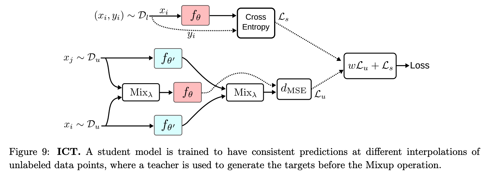
(9) Interpolation Consistency Training (ICT)

Random perturbations : inefficient in high dimensions

VAT and AdD :

• find the adversarial perturbations that will maximize the change in the model’s predictions

• problem : involves multiple forward and backward passes to compute these perturbations )

\(\rightarrow\) solution : propose Interpolation Consistency Training (ICT)

• efficient consistency regularization technique

Procedure

• MixUp operation : \(\operatorname{Mix}_\lambda(a, b)=\lambda \cdot a+(1-\lambda) \cdot b\)

  • outputs an interpolation between the two inputs with a weight \(\lambda \sim \operatorname{Beta}(\alpha, \alpha)\)
  • consider mixup as perturbation
    • \(x_i+\delta=\operatorname{Mix}_\lambda\left(x_i, x_j\right)\).

• prediction function \(f_\theta\)

  • consistent predictions at different interploations of \(x_i\) & \(x_j\)

    \(\rightarrow\) \(f_\theta\left(\operatorname{Mix}_\lambda\left(x_i, x_j\right)\right) \approx \operatorname{Mix}_\lambda\left(f_{\theta^{\prime}}\left(x_i\right), f_{\theta^{\prime}}\left(x_j\right)\right)\).

• targets are generated using a teacher model \(f_{\theta^{\prime}}\) ( = EMA of \(f_\theta\) )

unsupervised objective

• \(\mathcal{L}_u=w \frac{1}{ \mid \mathcal{D}_u \mid } \sum_{x_i, x_j \in \mathcal{D}_u} d_{\operatorname{MSE}}\left(f_\theta\left(\operatorname{Mix}_\lambda\left(x_i, x_j\right)\right), \operatorname{Mix}_\lambda\left(f_{\theta^{\prime}}\left(x_i\right), f_{\theta^{\prime}}\left(x_j\right)\right)\right.\).

benefit of ICT ( compared to random perturbations )

• consider mixup as perturbation
  • \(x_i+\delta=\operatorname{Mix}_\lambda\left(x_i, x_j\right)\).

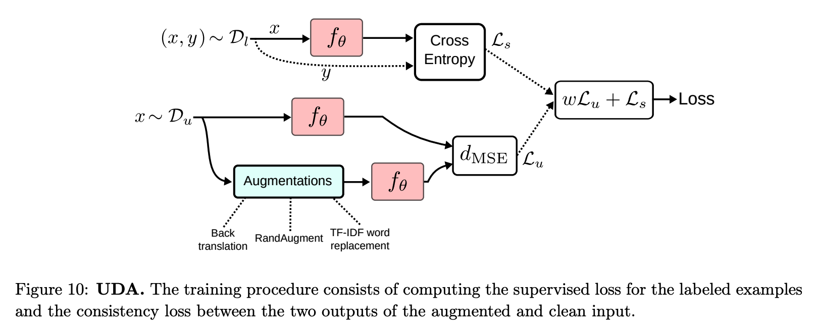
(10) Unsupervised Data Augmetnation

• ex 1) RandAugment for Image Classification.

• ex 2) Back-translation for Text Classification