
An Overview of Deep Semi-Supervised Learning (2020) - Part 3
Contents
- Abstract
- Introduction
- SSL
- SSL Methods
- Main Assumptions in SSL
- Related Problems
- Consistency Regularization
- Ladder Networks
- Pi-Model
- Temporal Ensembling
- Mean Teachers
- Dual Students
- Fast-SWA
- Virtual Adversarial Training (VAT)
- Adversarial Dropout (AdD)
- Interpolation Consistency Training (ICT)
- Unsupervised Data Augmentation
- Entropy Minimization
- Proxy-label Methods
- Self-training
- Multi-view Training
- Holistic Methods
- MixMatch
- ReMixMatch
- FixMatch
- Generative Models
- VAE for SSL
- GAN for SSL
- Graph-Based SSL
- Graph Construction
- Label Propagation
- Self-Supervision for SSL
6. Generative Models
Unsupervised Learning
- provided with \(x \sim p(x)\)
- objective : estimate the density
Supervised Learning
-
objective : find the relationship between \(x\) & \(y\)
- minimizing the functional \(p(x, y)\)
-
interested in the conditional distributions \(p(y \mid x)\),
( without the need to estimate \(p(x)\) )
Semi-supervised Learning with generative models
- extension of supervised / unsupervised learning
- information about \(p(x)\) provided by \(\mathcal{D}_u\)
- information of the provided labels from \(\mathcal{D}_l\)
(1) VAE for SSL
standard VAE
- autoencoder trained with a reconstruction loss
- + variational objective term
- attempts to learn a latent space that roughly follows a unit Gaussian distribution,
- implemented as the KL-divergence between latent space & standard Gaussian
Notation :
- input : \(x\)
- encoder : \(q_\phi(z \mid x)\)
- standard Gaussian distn : \(p(z)\)
- reconstructed input : \(\hat{x}\)
- decoder : \(p_\theta(x \mid z)\)
Loss Function :
- \(\mathcal{L}=d_{\mathrm{MSE}}(x, \hat{x})+d_{\mathrm{KL}}\left(q_\phi(z \mid x), p(z)\right)\).
a-1) Standard VAEs for SSL (M1 Model)
- consists of an unsupervised pretraining stage
- step 1) pre-train
- VAE is trained using the labeled and unlabeled examples
- step 2) standard supervised task
- 2-1) transform input \(x\)
- \(x \in \mathcal{D}_l\) are transformed into \(z\)
- 2-2) supervised task : \((z, y)\)
- 2-1) transform input \(x\)
- pros : classification can be performed in a lower dim
a-2) Extending VAEs for SSL (M2 Model)
- limitation of M1 model :
- labels of \(\mathcal{D}_l\) were ignored when training the VAE
- M2 model : also use label info
- 3 components
- (1) classification network : \(q_\phi(y \mid x)\)
- (2) encoder : \(q_\phi(z \mid y, x)\)
- (3) decoder : \(p_\theta(x \mid y, z)\)
- similar to a standard VAE …
- with the addition of the posterior on \(y\)
- loss terms to train \(q_\phi(y \mid x)\) if the labels are available
- \(q_\phi(y \mid x)\) : can then be used at test time to get the predictions on unseen data
a-3) Stacked VAEs (M1+M2 Model)
- concatenate M1 & M2
- procedures
- step 1) M1 is trained to obtain the \(z_1\)
- step 2) M2 uses the \(z_1\) from model M1 , instead of raw \(x\)
- final model :
- \(p_\theta\left(x, y, z_1, z_2\right)=p(y) p\left(z_2\right) p_\theta\left(z_1 \mid y, z_2\right) p_\theta\left(x \mid z_1\right)\).
b) Variational Auxiliary Autoencoder
extends the variational distn with auxiliary variables \(a\)
- \(q(a, z \mid x)=q(z \mid a, x) q(a \mid x)\).
pros : marginal distribution \(q(z \mid x)\) can fit more complicated posteriors \(p(z \mid x)\)
to have an unchanged generative model \(p(x \mid z)\)….
-
joint mode \(p(x,z,a)\) gives back the original \(p(x,z)\) under marginalization over \(a\)
\(\rightarrow\) \(p(x,z,a) = p(a \mid x,z)p(x,z)\) , with \(p(a \mid x, z) \neq p(a)\)
SSL setting : use class information
- additional latent variable \(y\) is introduced
- generative model : \(p(y) p(z) p(a \mid z, y, x) p(x \mid y, z)\)
- \(a\) : auxiliary variable
- \(y\) : class label
- \(z\) : latent features
- result : 5 NNs
- (1) auxiliary inference model : \(q(a \mid x)\)
- (2) latent inference model : \(q(z \mid a, y, x)\)
- (3) classifiaciton model : \(q(y \mid a, x)\)
- (4) generative model 1 : \(p(a \mid \cdot)\)
- (5) generative model 2 : \(p(x \mid \cdot)\)
(2) GAN for SSL
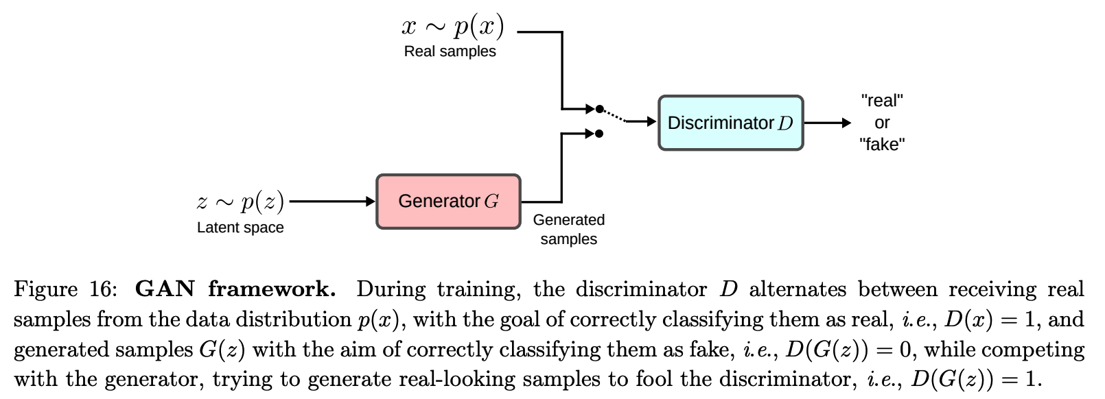
\(\begin{aligned} \mathcal{L}_D &=\max _D \mathbb{E}_{x \sim p(x)}[\log D(x)]+\mathbb{E}_{z \sim p(z)}[1-\log D(G(z))] \\ \mathcal{L}_G &=\min _G-\mathbb{E}_{z \sim p(z)}[\log D(G(z))] \end{aligned}\).
a) CatGAN (Categorical GAN)
GAN vs CatGAN
- GAN : real vs fake
- CatGAN : class 1 vs class2 vs … class K vs fake
combining both the generative & discriminative perspectives
- discriminator \(D\) plays the role of \(C\) classifiers
Objective :
- trained to maximize the mutual information between…
- (1) the inputs \(x\)
- (2) predicted labels for a number of \(C\) unknown classes
For Discriminator….
-
real data : one class label \(\rightarrow\) minimize \(H[p(y \mid x, D)]\)
-
fake data : no class \(\rightarrow\) maximize \(H[p(y\mid x, G(z))]\)
-
assumption that # of data of each class are even :
\(\rightarrow\) maximize \(H[p(y \mid D)]\)
For Generator ….
-
have to fool Discriminator that generated data belongs to certain class
\(\rightarrow\) minimize \(H[p(y\mid x, G(z))]\)
-
assumption that # of data of each class are even :
\(\rightarrow\) maximize \(H[p(y \mid D)]\)
Loss Function
\(\begin{aligned} \mathcal{L}_D &=\max _D-\mathbb{E}_{x \sim p(x)}[\mathrm{H}(D(x))]+\mathbb{E}_{z \sim p(z)}[\mathrm{H}(D(G(z)))]+\mathrm{H}_{\mathcal{D}} \\ \mathcal{L}_G &=\min _G \mathbb{E}_{z \sim p(z)}[\mathrm{H}(D(G(z)))]-\mathrm{H}_G \end{aligned}\).
- \(\mathrm{H}_{\mathcal{D}} =\mathrm{H}\left(\frac{1}{N} \sum_{i=1}^N D\left(x_i\right)\right)\).
- \(\mathrm{H}_G \approx \mathrm{H}\left(\frac{1}{M} \sum_{i=1}^M D\left(G\left(z_i\right)\right)\right)\).
SSL setting
- \(x\) comes from \(\mathcal{D}_l\)
- \(y\) comes in form of one-hot vector
Loss function of \(D\) :
- \(\mathcal{L}_D+\lambda \mathbb{E}_{(x, y) \sim p(x)_{\ell}}[-y \log G(x)]\).
b) DCGAN
build good image representations by training GANs
\(\rightarrow\) reuse parts of the \(G\) & \(D\) as feature extractors for supervised tasks
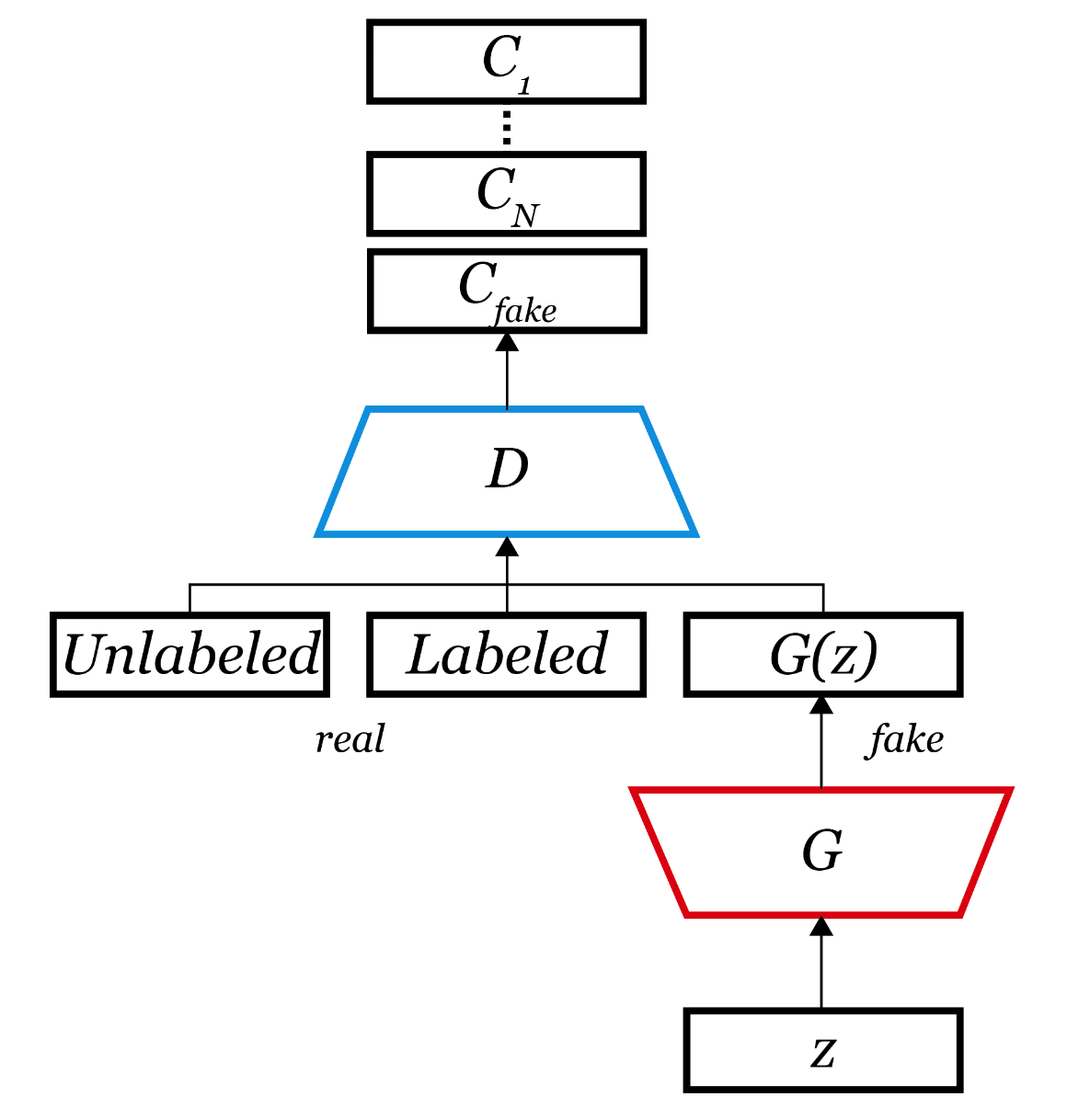
c) SGAN (Semi-Supervised GAN)
DCGAN : \(D\) & \(G\) improves alternatively
SGAN : does it simultaneously!
-
instead of real/fake discrimination, has \(C+1\) outputs!
( sigmoid \(\rightarrow\) softmax )
-
architecture : same as DCGAN
d) Feature Matching GAN
Feature Matching
- Instead of directly maximizing the output of the discriminator…
\(\rightarrow\) requires the \(G\) to generate data that matches the first-order feature statistics between of the data distribution
Example ) intermediate layer :
- \(\mid \mid \mathbb{E}_{x \sim p(x)}[h(x)]-\mathbb{E}_{z \sim p(z)}[h(G(z))] \mid \mid ^2\).
Still have the problem of generator mode collapse!
\(\rightarrow\) minibatch discrimination
( = allow the discriminator to look at multiple data examples in combination )
SSL settings
- \(D\) in feature matching GAN employs a \((C+1)\)-classification ( instead of binary classification )
- the prob of \(x\) being fake : \(p(y=C+1 \mid G(z), D)\)
- ( = \(1-D(x)\) in the original GAN )
- Loss function : \(\mathcal{L}=\mathcal{L}_s+\mathcal{L}_u\)
- \(\mathcal{L}_s =-\mathbb{E}_{x, y \sim p(x)_l}[\log p(y \mid x, y<K+1, D)]\).
- \(\mathcal{L}_u =-\mathbb{E}_{x \sim p(x)_u} \log \ [1-p(y=K+1 \mid x, D)]-\mathbb{E}_{z \sim p(z)} \log \ [p(y=K+1 \mid G(z), D))]\).