
An Overview of Deep Semi-Supervised Learning (2020) - Part 2
Contents
- Abstract
- Introduction
- SSL
- SSL Methods
- Main Assumptions in SSL
- Related Problems
- Consistency Regularization
- Ladder Networks
- Pi-Model
- Temporal Ensembling
- Mean Teachers
- Dual Students
- Fast-SWA
- Virtual Adversarial Training (VAT)
- Adversarial Dropout (AdD)
- Interpolation Consistency Training (ICT)
- Unsupervised Data Augmentation
- Entropy Minimization
- Proxy-label Methods
- Self-training
- Multi-view Training
- Holistic Methods
- MixMatch
- ReMixMatch
- FixMatch
- Generative Models
- VAE for SSL
- GAN for SSL
- Graph-Based SSL
- Graph Construction
- Label Propagation
- Self-Supervision for SSL
3. Entropy Minimization
-
encourage the network to make confident (i.e., low-entropy) predictions on unlabeled data
-
by adding a loss term which minimizes the entropy of the prediction function \(f_\theta(x)\)
- ex) categorical output space with \(C\) classes : \(-\sum_{k=1}^C f_\theta(x)_k \log f_\theta(x)_k\).
However …model can quickly overfit to low confident data
\(\rightarrow\) entropy minimization doesn’t produce competitive results compared to other SSL methods
( but can produce state-of-the-art results when combined with different approaches )
4. Proxy-label Methods
(1) Self-training
Procedure
-
step 1) small amount of labeled data \(D_l\) is first used to train a prediction function \(f_{\theta}\)
-
step 2) \(f_{\theta}\) is used to assign pseudo-labels to \(x \in D_u\)
-
confidence above pre-determined threshold \(\tau\)
( Other heuristics can be used .
ex) using the relative confidence instead of the absolute confidence )
-
Impact of self-training \(\approx\) entropy minimization
- both forces to output more confident predictions
The main downside of such methods : unable to correct its own mistake
Meta Pseudo Labels
- student-teacher setting
- teacher : produce the proxy labels
- based on an efficient meta-learning algorithm called Meta Pseudo Labels (MPL)
- updated by policy gradients
- encourages the teacher to adjust the target distns of training examples in a way that improves the learning of the student model
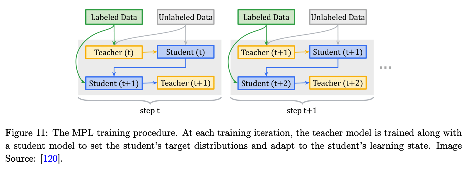
Procedure
- step 1) Student learns from the Teacher
- given a single input example \(x \in D_l\), teacher \(f_{\theta^{'}}\) produces a target class-distn to train student \(f_{\theta}\)
- the student is shown \((x, f_{\theta^{'}}(x))\) & update its parameters
- step 2) Teacher learns from the Student
- new parameter \(\theta(t+1)\) are evaluated on an example \((x_{val}, y_{val})\)
(2) Multi-view Training
utilizes multi-view data
- different views can be collected by …
- different measuring methods
- creating limited views of the original data
Notation
- prediction function : \(f_{\theta_i}\)
- view of \(x\) : \(v_i(x)\)
a) Co-training
- 2 conditionally independent views \(v_1(x)\) and \(v_2(x)\)
- 2 prediction functions \(f_{\theta_1}\) and \(f_{\theta_2}\)
- trained on a specific view on the labeled set \(\mathcal{D}_l\)
Step 1) train \(f_{\theta_1}\) and \(f_{\theta_2}\) on \(\mathcal{D}_l\)
Step 2) Proxy Labeling
- unlabeled data is added to the training set of the \(f_{\theta_i}\) if \(f_{\theta_j}\) outputs a confident prediction
etc
- different learning algorithms to learn two different classifiers OK
- two views \(v_1(x)\) and \(v_2(x)\) can be generated by injecting noise or DA
Democratic Co-training
- replacing the different views of the input data with a number of models with different architectures and learning algorithms
- trained models are then used to label a given example x if a majority of models confidently agree on its label.
b) Tri-Training
- to overcome the lack of data with multiple views
- utilize the agreement of 3 independently trained models
Procedure
- step 1) \(\mathcal{D}_l\) is used to train \(f_{\theta_1}\), \(f_{\theta_2}\), \(f_{\theta_3}\)
- step 2) \(x \in \mathcal{D}_u\) is then added to the training set of the function \(f_{\theta_i}\)
- if the other 2 models agree on its predicted label
- step 3) training stops if no data points are being added
Pros : generally applicable!
- requires neither the existence of multiple views nor unique learning algorithms
Cons : using with NN \(\rightarrow\) expensive
-
propose to sample a limited number of unlabeled data at each training epoch
( the candidate pool size is increased as the training progresses )
Multi-task tri-training
-
used to reduce the time and sample complexity
-
all three models share the same feature-extractor with model-specific classification layers
-
ex) Tri-Net
Cross-View training
- (previous works) self-training
- model plays a dual role of a teacher and a student
- inspiration from multi-view learning and consistency training
- model is trained to produce consistent predictions across different views of the inputs
- Instead of using a single model as a teacher and a student…
- use a shared encoder & auxiliary prediction modules
- auxiliary prediction modules
- (1) auxiliary student modules
- (2) primary teacher module
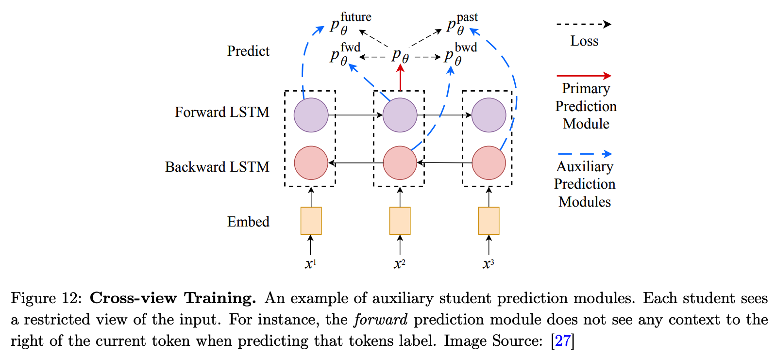
- primary teacher module :
- trained only on labeled examples
- generate the pseudo-labels, by taking as input the full view of the unlabeled inputs
- student modules:
- trained to have consistent predictions with the teacher module
Loss fuction
- \(\mathcal{L}=\mathcal{L}_u+\mathcal{L}_s=\frac{1}{ \mid \mathcal{D}_u \mid } \sum_{x \in \mathcal{D}_u} \sum_{i=1}^K d_{\mathrm{MSE}}\left(t(e(x)), s_i(e(x))\right)+\frac{1}{ \mid \mathcal{D}_l \mid } \sum_{x, y \in \mathcal{D}_l} \mathrm{H}(t(e(x)), y)\).
- encoder : \(e\)
- teacher module : \(t\)
- \(K\) student modules : \(s_i\) ( where \(i \in [0,K]\) )
- receives only a limited view of the input
The student can learn from the teacher
\(\because\) teacher : UNlimited view & student : limited view
5. Holistic Methods
unify dominant methods in SSL in a single framework
(1) MixMatch
Input
- batch from \(\mathcal{D}_l\)
- batch from \(\mathcal{D}_u\)
- hyperparameters
- sharpening temperature \(T\)
- number of augmentations \(K\)
- Beta distn parameter \(\alpha\)
Output
- batch of augmented labeled examples
- batch of augmented unlabeled examples + proxy labels
\(\rightarrow\) can be used to compute the losses
Procedure
-
step 1) Data Augmentation
- \(\tilde{x}_1, \ldots, \tilde{x}_K\).
-
step 2) Label Guessing
- producing proxy labels
- step 2-1) generate the predictions for \(\tilde{x}_1, \ldots, \tilde{x}_K\)
- step 2-2) average the predictions : \(\hat{y}=1 / K \sum_{k=1}^K\left(\hat{y}_k\right)\)
- result : \(\left(\tilde{x}_1, \hat{y}\right), \ldots,\left(\tilde{x}_K, \hat{y}\right)\).
- producing proxy labels
-
step 3) Sharpening
- to produce confident predictions
- \((\hat{y})_k=(\hat{y})_k^{\frac{1}{T}} / \sum_{k=1}^C(\hat{y})_k^{\frac{1}{T}}\).
-
step 4) MixUp
- Notation
- \(\mathcal{L}\) : augmented labeled data
- \(\mathcal{U}\) : augmented unlabeled data + proxy labels
- \(K\) times larger than the original batch!
- step 1) mix these 2 batches
- \(\mathcal{W}=\operatorname{Shuffle}(\operatorname{Concat}(\mathcal{L}, \mathcal{U}))\).
- step 2) divide \(\mathcal{W}\)
- (1) \(\mathcal{W}_1\) : same size as \(\mathcal{L}\)
- (2) \(\mathcal{W}_2\) : same size as \(\mathcal{U}\)
- step 3) Mixup operation ( + modification )
- \(\mathcal{L}^{\prime}=\operatorname{MixUp}\left(\mathcal{L}, \mathcal{W}_1\right)\).
- \(\mathcal{U}^{\prime}=\operatorname{MixUp}\left(\mathcal{U}, \mathcal{W}_2\right)\).
- Notation
Loss Function
- standard SSL losses
- CE loss ( supervised )
- Consistency loss ( unsupervised )
- \(\mathcal{L}=\mathcal{L}_s+w \mathcal{L}_u=\frac{1}{ \mid \mathcal{L}^{\prime} \mid } \sum_{x, y \in \mathcal{L}^{\prime}} \mathrm{H}\left(y, f_\theta(x)\right)+w \frac{1}{ \mid \mathcal{U}^{\prime} \mid } \sum_{x, \hat{y} \in \mathcal{U}^{\prime}} d_{\mathrm{MSE}}\left(\hat{y}, f_\theta(x)\right)\).
(2) ReMixMatch
improve MixMatch by introducing 2 new techniques :
- (1) distribution alignment
- (2) augmentation anchoring
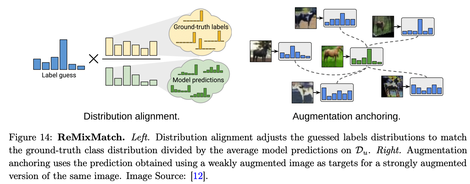
a) Distribution alignment
-
encourages the marginal distn of predictions on unlabeled data to be close to the marginal distn of GT labels
-
ex) given prediction result \(f_\theta(x)\) …
\(\rightarrow\) \(f_\theta(x)=\operatorname{Normalize}\left(f_\theta(x) \times p(y) / \tilde{y}\right)\)
b) Augmentation anchoring
-
feeds multiple strongly augmented versions of the input into the model
& encourage each output to be close to the prediction for a weakly-augmented version of the same input
-
model’s prediction for a weakly augmented version = proxy label
Loss Function
\(\mathcal{L}=\mathcal{L}_s+w \mathcal{L}_u=\frac{1}{ \mid \mathcal{L}^{\prime} \mid } \sum_{x, y \in \mathcal{L}^{\prime}} \mathrm{H}\left(y, f_\theta(x)\right)+w \frac{1}{ \mid \mathcal{U}^{\prime} \mid } \sum_{x, \hat{y} \in \mathcal{U}^{\prime}} \mathrm{H}\left(\hat{y}, f_\theta(x)\right)\),
Also add a self-supervised loss
- new unlabeled batch \(\hat{\mathcal{U}}^{\prime}\) of examples is created
- by rotating all of the examples with an angle \(r \sim\{0,90,180,270\}\). T
- \(\mathcal{L}_{S L}=w^{\prime} \frac{1}{ \mid \hat{\mathcal{U}}^{\prime} \mid } \sum_{x, \hat{y} \in \hat{\mathcal{U}}^{\prime}} \mathrm{H}\left(\hat{y}, f_\theta(x)\right)+\lambda \frac{1}{ \mid \hat{\mathcal{U}}^{\prime} \mid } \sum_{x \in \hat{\mathcal{U}}^{\prime}} \mathrm{H}\left(r, f_\theta(x)\right)\).
(3) FixMatch
simple SSL algorithm, that combines
- (1) consistency regularization
- (2) pseudo-labeling
both the supervised & unsupervised losses : CE Loss
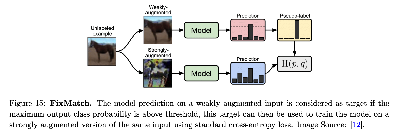
Labeled & Unlabeled
- Labeled : just use gt
- Unlabeled :
- step 1) 1 weakly augmented version is computed
- Weak augmentation function : \(A_w\)
- step 2) predict it & use it as proxy label
- if confidence > \(\tau\)
- step 3) \(K\) strongly augmented versions are computed
- step 1) 1 weakly augmented version is computed
Unsupervised Loss :
- \(\mathcal{L}_u=w \frac{1}{K \mid \mathcal{D}_u \mid } \sum_{x \in \mathcal{D}_u} \sum_{i=1}^K 1\left(\max \left(f_\theta\left(A_w(x)\right)\right) \geq \tau\right) \mathrm{H}\left(f_\theta\left(A_w(x)\right), f_\theta\left(A_s(x)\right)\right)\).