(paper 99) Deep Adaptive Input Normalization for Price Forecasting using Limit Order Book Data

Deep Adaptive Input Normalization for Price Forecasting using Limit Order Book Data (2019)

https://github.com/passalis/dain.

Contents

1. Abstract
2. Introduction
3. DAIN

Abstract

DAIN

• simple, yet effective, neural layer
• capable of adaptively normalizing the input time series

• take into account the distribution of the data

• trained in an end-to-end fashion using back-propagation

Key point

“learns how to perform normalization for a given task, instead of using a fixed normalization scheme”

• can be directly applied to any new TS without requiring re-training

1. Introduction

Deep Adaptive Input Normalization (DAIN): capable of

• a) learning how the data should be normalized
• b) adaptively changing the applied normalization scheme during inference
  • according to the distribution of the measurements of the current TS

\(\rightarrow\) effectively handle non-stationary and multimodal data

3 sublayers

• (layer 1: centering) shifting the data
• (layer 2: standardization) linearly scaling the data
• (layer 3: gating) performing gating, i.e., nonlinearly suppressing features that are irrelevant or not useful

\(\rightarrow\) the applied normalization is TRAINABLE

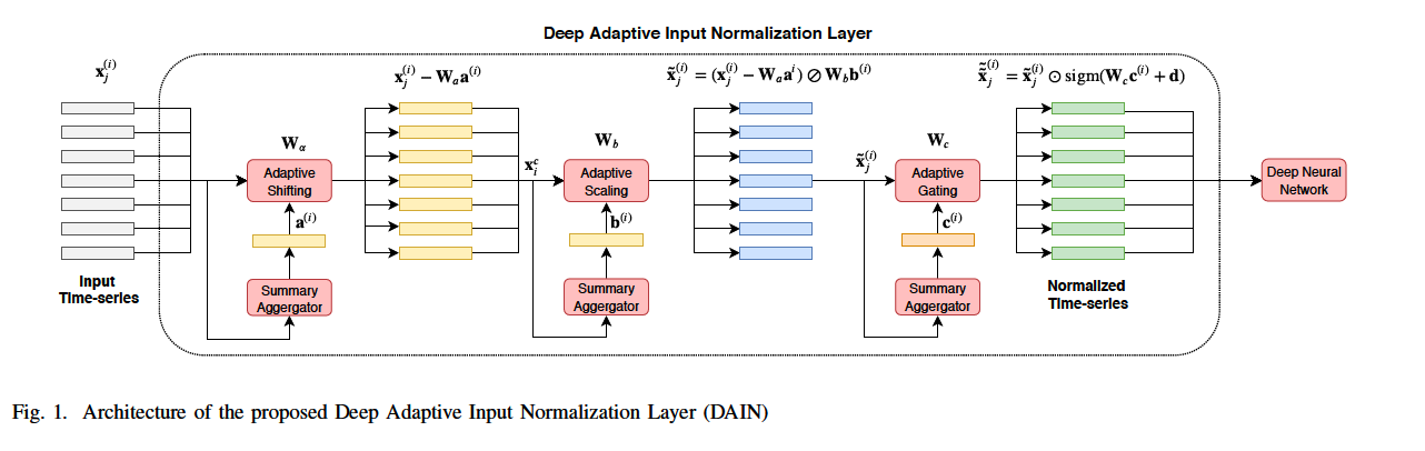
2. Deep Adaptive Input Normalization (DAIN)

\(N\) time series: \(\left\{\mathbf{X}^{(i)} \in \mathbb{R}^{d \times L} ; i=1, \ldots, N\right\}\)

• \(\mathbf{x}_j^{(i)} \in \mathbb{R}^d, j=1,2, \ldots, L\) : \(d\) features observed at time point \(j\) in time series \(i\).

Z-score normalization

• most widely used form of normalization

• if data were not generated by a unimodal Gaussian distribution…

  \(\rightarrow\) lead to sub-optimal results

  \(\rightarrow\) should be normalized in an mode-aware fashion

Goal : learn how to shift & scale

• \(\tilde{\mathbf{x}}_j^{(i)}=\left(\mathbf{x}_j^{(i)}-\boldsymbol{\alpha}^{(i)}\right) \oslash \boldsymbol{\beta}^{(i)}\).

• ex) z-score normalization

  • \(\boldsymbol{\alpha}^{(i)}=\) \(\boldsymbol{\alpha}=\left[\mu_1, \mu_2, \ldots, \mu_d\right]\) and \(\boldsymbol{\beta}^{(i)}=\boldsymbol{\beta}=\left[\sigma_1, \sigma_2, \ldots, \sigma_d\right]\),
    • where \(\mu_k\) and \(\sigma_k\) refer to the global average and standard deviation of the \(k\)-th input feature

Procedure

• step 1-1) summary representation of the TS
  • \(\mathbf{a}^{(i)}=\frac{1}{L} \sum_{j=1}^L \mathbf{x}_j^{(i)} \in \mathbb{R}^d\).
    • average all the \(L\) measurements
  • provides an initial estimation for the mean
• step 1-2) generate shifting operator \(\boldsymbol{\alpha}^{(i)}\)
  • \(\boldsymbol{\alpha}^{(i)}=\mathbf{W}_a \mathbf{a}^{(i)} \in \mathbb{R}^d\).
    • linear transformation of \(\mathbf{a}^{(i)}\)
    • where \(\mathbf{W}_a \in \mathbb{R}^{d \times d}\) is the weight matrix of the first NN layer
  • ( called adaptive shifting layer )
    • \(\because\) estimates how the data must be shifted before feeding them to the network.
  • allows for exploiting possible correlations between different features to perform more robust normalization.

• step 2-1) update (2nd) summary representations

  • \(b_k^{(i)}=\sqrt{\frac{1}{L} \sum_{j=1}^L\left(x_{j, k}^{(i)}-\alpha_k^{(i)}\right)^2}, \quad k=1,2, \ldots, d\).

    ( corresponds to stddev )

• step 2-2) generate scaling operator \(\boldsymbol{\beta}^{(i)}\)
  • \(\boldsymbol{\beta}^{(i)}=\mathbf{W}_b \mathbf{b}^{(i)} \in \mathbb{R}^d\).
    • where \(\mathbf{W}_b \in \mathbb{R}^{d \times d}\) is the weight matrix the scaling layer
  • ( called adaptive scaling layer )
    • \(\because\) estimates how the data must be scaled before feeding them to the network.
• step 2-3) normalize using \(\alpha\) and \(\beta\)
  • \(\tilde{\mathbf{x}}_j^{(i)}=\left(\mathbf{x}_j^{(i)}-\boldsymbol{\alpha}^{(i)}\right) \oslash \boldsymbol{\beta}^{(i)}\).

• step 3) adaptive gating layer

  • suppressing features that are not relevant or useful
  • \(\tilde{\tilde{\mathbf{x}}}_j^{(i)}=\tilde{\mathbf{x}}_j^{(i)} \odot \gamma^{(i)}\),
    • where \(\gamma^{(i)}=\operatorname{sigm}\left(\mathbf{W}_c \mathbf{c}^{(i)}+\mathbf{d}\right) \in \mathbb{R}^d\)
      • where \(\mathbf{W}_c \in\) \(\mathbb{R}^{d \times d}\) and \(\mathbf{d} \in \mathbb{R}^d\) are the parameters of the gating layer
      • where \(\mathbf{c}^{(i)}\) is a (3rd) summary representation : \(\mathbf{c}^{(i)}=\frac{1}{L} \sum_{j=1}^L \tilde{\mathbf{x}}_j^{(i)} \in \mathbb{R}^d\)

Summary: \(\alpha^{(i)}, \beta^{(i)}, \gamma^{(i)}\) are dependent on ..

• current ‘local’ data on window \(i\)
• ‘global’ estimates of \(\mathbf{W}_a, \mathbf{W}_b, \mathbf{W}_c, \mathbf{d}\)