
Discrete Fourier Transform
참고 : https://www.youtube.com/watch?v=fMqL5vckiU0&list=PL-wATfeyAMNrtbkCNsLcpoAyBBRJZVlnf
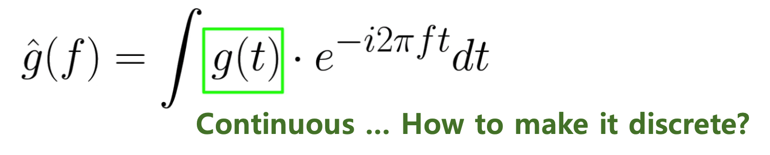
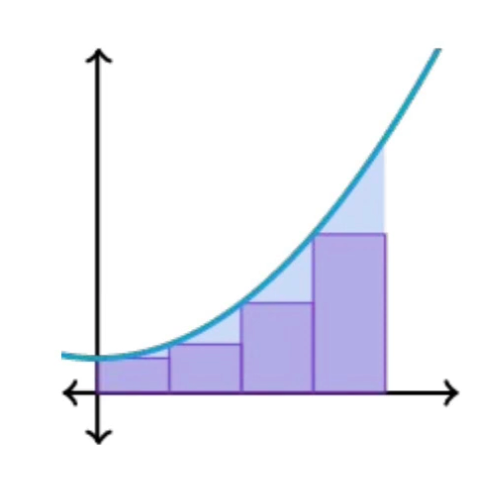
1. Continuous vs. Discrete
We have to handle it in discrete space.
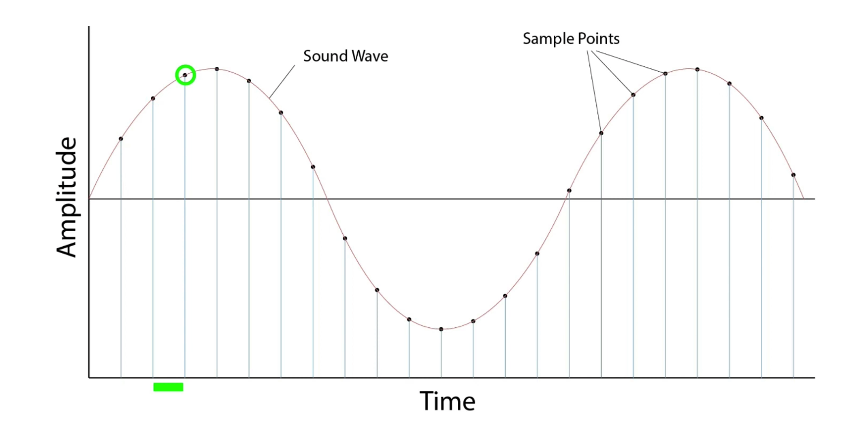
ex) Digitalization
- by sampling at interval
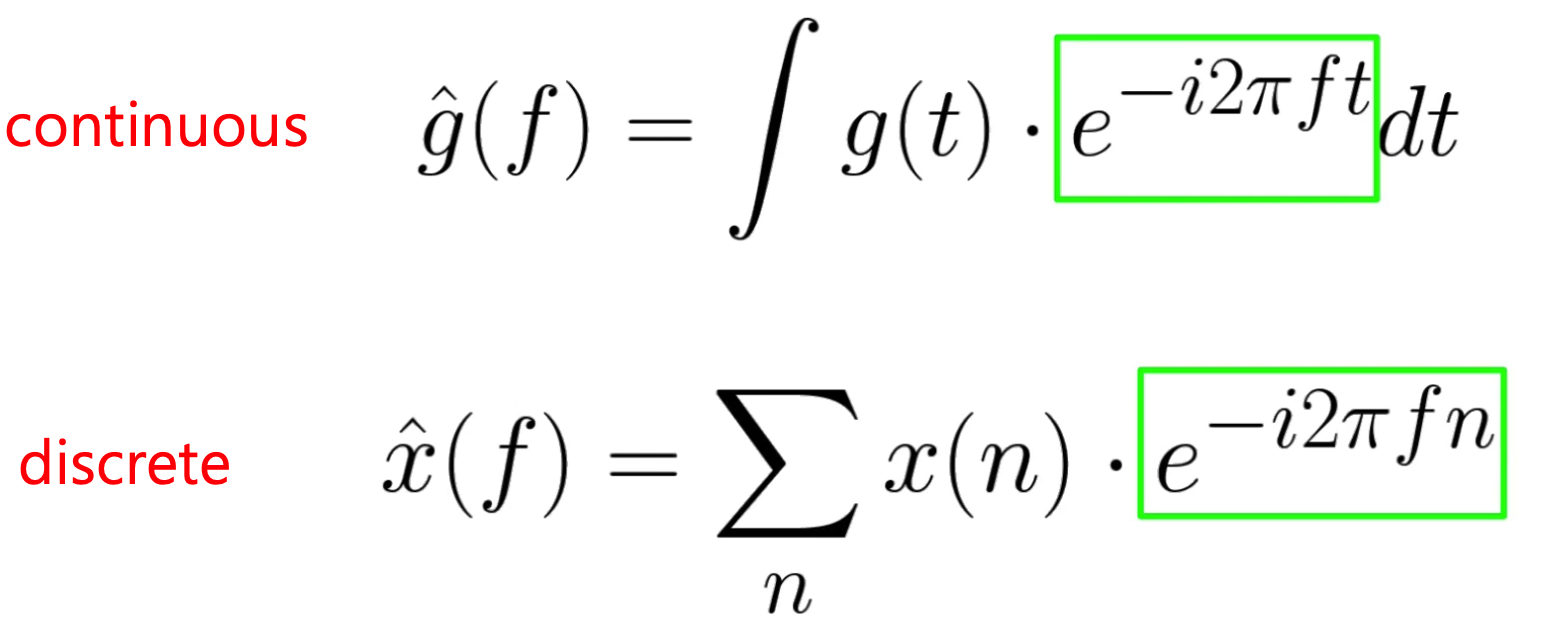
2. DFT
\(\hat{x}(f)=\sum_n x(n) \cdot e^{-i 2 \pi f n}\).
Solution 1) Time
consider \(f\) to be a non-zero FINITE time interval
- \(x(0), \cdots x(N-1)\).
Solution 2) Frequency
compute transform for FINITE number of frequencies
number of frequency (\(M\)) = number of samples (\(N\))
- why same?
- (1) inversible transformation
- (2) computational efficiency
Result:
\(\hat{x}(k / N)=\sum_{n=0}^{N-1} x(n) \cdot e^{-i 2 \pi n \frac{k}{N}}\).
- \(\int \rightarrow\) \(\sum_{n=1}^{N-1}\) : solution 1)
- \(f \rightarrow\) \(k/N\) : solution 2)
- where \(k=[0, M-1]=[0, N-1]\)
\(f \approx F(k)=\frac{k}{N T}=\frac{k s_r}{N}\).
- \(k\) : frequency of \(k\) ( = Hz)
- \(T\) : sampling period
- \(N\) : number of samples
- \(s_r\) : sampling rate ( = inverse of \(T\) )
3. Redundancy in DFT
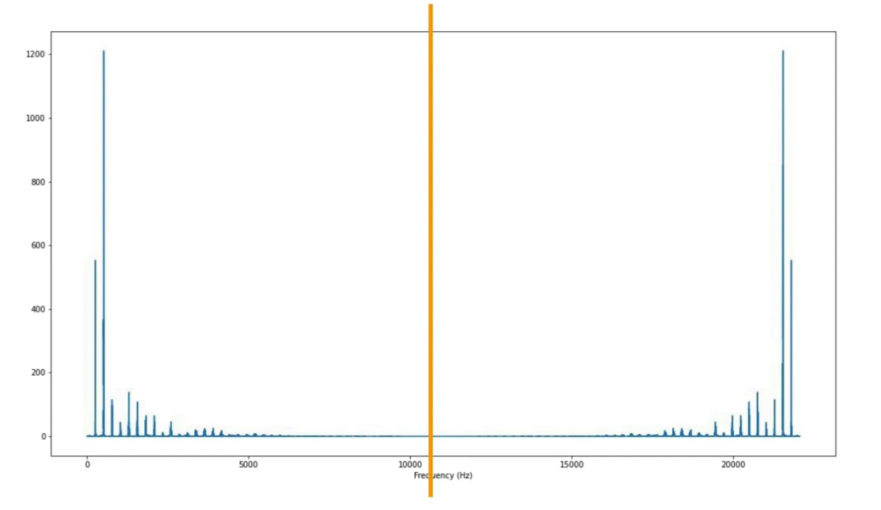
- Symmetric!
Symmetric on \(k=N/2\) … Why?
\(k=N/2\) \(\rightarrow\) \(f \approx F(k) = F(N/2) = s_r/2\)
This means that we only have to look at the left hand part!
DFT \(\rightarrow\) Fast FT (FFT)
DFT : \(O(N^2)\)
FFT : \(O(N \log_2 N)\)
\(\rightarrow\) by exploiting redundancies!
( limitation: FFT works when \(N\) is a power of \(2\) )