
Multivariate Probabilistic Time Series Forecasting via Conditioned Normalizing Flows (2021)
Contents
- Abstract
- Introduction
- Background
- Density Estimation via NF
- Self-Attention
- Temporal Conditioned NF
- RNN Conditioned Real NVP
- Transformer Conditioned Real NVP
- Training
- Training
- Covariates
0. Abstract
여러 time series 존재 시, 쉽게 푸는 법 : Independence 가정?
\(\rightarrow\) ignore “interaction effect”
DL 방법론들을 통해 위 interaction 포착 O…
BUT multivariate models often assume a simple parametric distn & do not scale to high dim
[ Proposal ]
model the multivariate temporal dynamics of t.s via Autoregressive DL model,
where data distn is represented by conditioned NF(Normalizing Flow)
1. Introduction
(1) Classical t.s
- univariate forecast
- require hand-tuned features
(2) DL t.s
- RNN ( LSTM, GRU )
- popular due to ..
- 1) ‘end-to-end’ training
- 2) incorporating exogenous covariates
- 3) automatic feature xtraction
Output can be
- (a) deterministic ( = point estimation )
- (b) probabilistic
\(\rightarrow\) w.o probabilistic modeling, the importance of the forecast in regions of “low noise” vs “high noise” cannot be distinguished
Proposal
end-to-end trainable AUTOREGRESSIVE DL architecture for PROBABILISTIC FORECASTING
that explicitly models MTS and their temporal dynamics by employing NORMALIZING FLOWS ( ex. MAF, Real NVP )
2. Background
(1) Density Estimation via NF
NF (Normalizing Flow)
-
mapping \(\mathbb{R}^{D}\) \(\rightarrow\) \(\mathbb{R}^{D}\)
-
\(f: \mathcal{X} \mapsto \mathcal{Z}\) : composed of a sequence of bijections or invertible functions
-
change of variables formula :
\(p_{\mathcal{X}}(\mathbf{x})=p_{\mathcal{Z}}(\mathbf{z}) \mid \operatorname{det}\left(\frac{\partial f(\mathbf{x})}{\partial \mathbf{x}}\right) \mid\).
-
inverse (should be) easy to evaluate ( \(\mathbf{x}=f^{-1}(\mathbf{z})\) )
-
computing Jacobian determinant takes \(O(D)\) time
ex) Real NVP (2017)
-
use coupling layer
-
\(\left\{\begin{array}{l} \mathbf{y}^{1: d}=\mathbf{x}^{1: d} \\ \mathbf{y}^{d+1: D}=\mathbf{x}^{d+1: D} \odot \exp \left(s\left(\mathbf{x}^{1: d}\right)\right)+t\left(\mathbf{x}^{1: d}\right) \end{array}\right.\).
-
change of variables formula :
\(\log p_{\mathcal{X}}(\mathbf{x})=\log p_{\mathcal{Z}}(\mathbf{z})+\log \mid \operatorname{det}(\partial \mathbf{z} / \partial \mathbf{x}) \mid =\log p_{\mathcal{Z}}(\mathbf{z})+\sum_{i=1}^{K} \log \mid \operatorname{det}\left(\partial \mathbf{y}_{i} / \partial \mathbf{y}_{i-1}\right) \mid .\).
-
Jacobian = “block-triangular matrix”
\(\therefore\) \(\log \mid \operatorname{det}\left(\partial \mathbf{y}_{i} / \partial \mathbf{y}_{i-1}\right) \mid =\log \mid \exp \left(\operatorname{sum}\left(s_{i}\left(\mathbf{y}_{i-1}^{1: d}\right)\right) \mid\right.\)
-
maximize average log likelihood, \(\mathcal{L}=\frac{1}{ \mid \mathcal{D} \mid } \sum_{\mathbf{x} \in \mathcal{D}} \log p_{\mathcal{X}}(\mathbf{x} ; \theta)\).
ex) MAF (Masked Autoregressive Flows) (2017)
-
generalization of Real NVP
-
transformation layer = “AUTOREGRESSIVE” NN
\(\rightarrow\) makes the Jacobian Triangular \(\rightarrow\) reduce computational cost ( tractable Jacobian! )
(2) Self-Attention
Transformer’s self-attention
\(\rightarrow\) enables to capture both long & short-term dependencies
\(\mathbf{O}_{h}=\operatorname{Attention}\left(\mathbf{Q}_{h}, \mathbf{K}_{h}, \mathbf{V}_{h}\right)=\operatorname{softmax}\left(\frac{\mathbf{Q}_{h} \mathbf{K}_{h}^{\top}}{\sqrt{d_{K}}} \cdot \mathbf{M}\right) \mathbf{V}_{h}\).
3. Temporal Conditioned NF
Notation
- MTS : \(x_{t}^{i} \in \mathbb{R}\) for \(i \in\{1, \ldots, D\}\) ( \(t\) = time index )
- \(\mathbf{x}_{t} \in \mathbb{R}^{D}\).
- \(i \in\{1, \ldots, D\}\).
- \(t\) = time index
- (for training) split this time seires by..
- 1) context window \(\left[1, t_{0}\right)\)
- 2) prediction window \(\left[t_{0}, T\right]\)
Simple model for MTS data : using “factorizing distn” in the emission model
-
shared param : learn patterns across individual time series
-
to capture dependencies…. “full joint distn”
\(\rightarrow\) BUT, full covariance matrix :
- number of param in NN : \(O\left(D^{2}\right)\)
- computing loss is TOO expensive
Wish to have a “SCALABLE” model & flexible distn model on the emission
\(\rightarrow\) model the conditional joint distn at time \(t\) of all time series \(p_{\mathcal{X}}\left(\mathbf{x}_{t} \mid \mathbf{h}_{t} ; \theta\right)\) with NF, conditioned on either the hidden state of RNN at time \(t\), or an embedding of t.s up to \(t-1\) from attention module
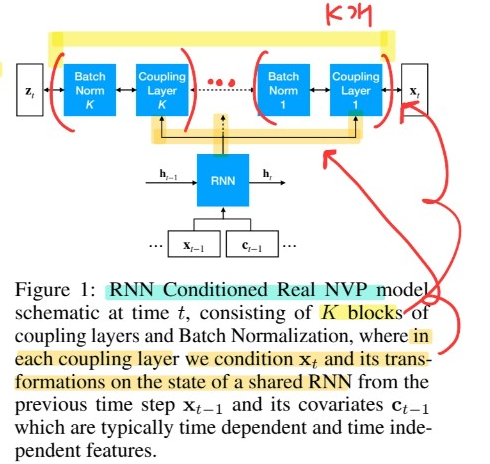
(1) RNN Conditioned Real NVP
Ex) autoregressive RNN (LSTM,GRU)..
- \(\mathbf{h}_{t}=\mathrm{RNN}\left(\operatorname{concat}\left(\mathbf{x}_{t-1}, \mathbf{c}_{t-1}\right), \mathbf{h}_{t-1}\right)\).
For powerful emission distn model… “stack \(K\) layers” of conditional flow ( Real NVP, MAF … )
-
\(p_{\mathcal{X}}\left(\mathbf{x}_{t_{0}: T} \mid \mathbf{x}_{1: t_{0}-1}, \mathbf{c}_{1: T} ; \theta\right)=\Pi_{t=t_{0}}^{T} p_{\mathcal{X}}\left(\mathbf{x}_{t} \mid \mathbf{h}_{t} ; \theta\right)\).
( \(\theta\) : set of all param of both flow & RNN )
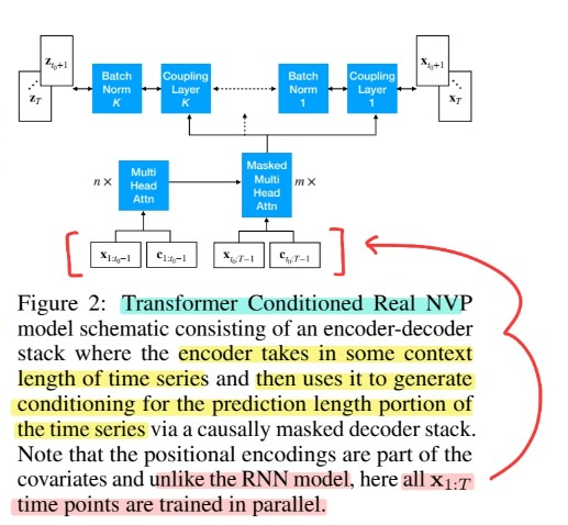
(2) Transformer Conditioned Real NVP
using Transformer
\(\rightarrow\) allows the model to “access any part of historic time series”, regardless of temporal distnace
( better than RNN! )
4. Training
(1) Training
maximize log-likelihood ( given in [2. Background] )
- \(\mathcal{L}=\frac{1}{ \mid \mathcal{D} \mid T} \sum_{\mathbf{x}_{1: T} \in \mathcal{D}} \sum_{t=1}^{T} \log p_{\mathcal{X}}\left(\mathbf{x}_{t} \mid \mathbf{h}_{t} ; \theta\right)\).
-
time series \(\mathbf{x}_{1:T}\) in batch \(D\) are selected from a random time window of size \(T\)
( + this increases the size of training data)
-
absolute time is only available to RNN/Transformer via the “covariates”
( not the relative position of \(x_t\) in training data )
Computational complexity
- Transformer : \(O\left(T^{2} D\right)\)
- RNN : \(O\left(T D^2 \right)\)
\(\rightarrow\) for \(D>T\) ( large multivariate time series ) … Transformer has much smaller complexity!
(2) Covariates
- use embeddings from “categorical features”
- covariates \(\mathbf{c}_t\)
- 1) time-dependent ( ex. 요일, 시 등 )
- 2) time-independent
- all covariates “are KNOWN” for time periods we want to forecast