(paper) DPSOM ; Deep Probabilistic Clustering with Self-Organizing Maps

DPSOM : Deep Probabilistic Clustering with Self-Organizing Maps (2020)

Contents

1. Abstract
2. Introduction
3. Probabilistic clustering with DPSOM
   1. Background
   2. PSOM : Probabilistic SOM clustering
   3. DPSOM : VAE for representation learning
   4. T-DPSOM : Extension to time series data

0. Abstract

interpretable visualizations from complex data :

• 1) clustering
• 2) representation learning

however, current methods do not combine those well!

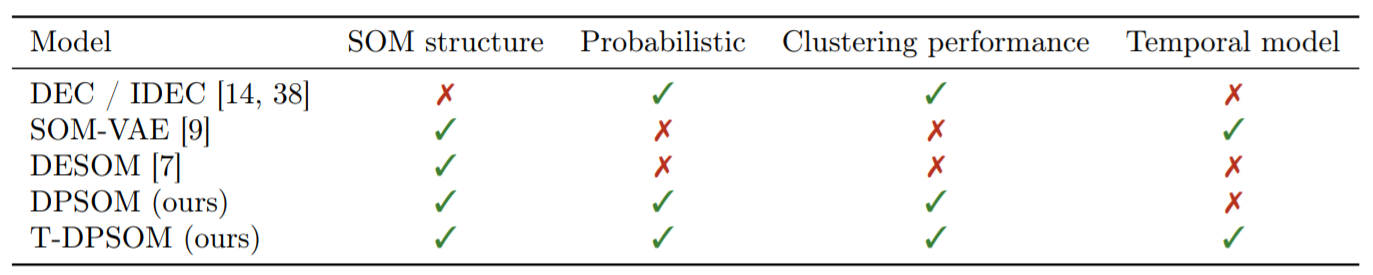
present a novel way to ..

• (a) fit SOM with probabilistic cluster assignments ( = PSOM )
• (b) new deep architecture for probabilistic clustering ( = DPSOM )
• (c) extend our architecture for ts clustering ( = T-DPSOM )

1. Introduction

[1] k-means, GMM

• constrained to simple data
• limited in high-dim / complex / real world data

[2] AE, VAE, GAN

• have been used in combination with clustering methods
• compressed latent representation : ease clustering process!

[3] SOM (Self-Organizing Map)

• interpretable representation
• low-dim ( usualy 2d ), discretized representations
• performs poorly on complex high-dim data
• effective for data viz / but few have been combined with DNN

to address issues in [3] SOM,

\(\rightarrow\) propose PSOM / DPSOM / T-DPSOM

2. Probabilistic clustering with DPSOM

Notation

• data samples \(\left\{x_{i}\right\}_{i=1, \ldots, N}\), where \(x_{i} \in \mathbb{R}^{d}\)
• goal : partition the data into a set of clusters \(\left\{S_{j}\right\}_{j=1, \ldots, K}\)

Proposed architecture

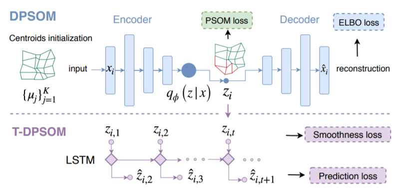
[ DPSOM ]

• use VAE to \(x \rightarrow z\)
• use PSOM to cluster \(z\)
• VAE & PSOM are trained jointly

[ T-DPSOM ]

• \(z_{i,,t}\) for \(t=1,..,T\) are connected by LSTM

  ( predict embedding \(z_{t+1}\) )

2-1. Background

SOM is comprised of \(K\) nodes : \(M=\left\{m_{j}\right\}_{j=1}^{K}\)

• node \(m_{j}\) corresponds to a centroid \(\mu_{j}\) in the input space

Algorithm

• randomly selects an input \(x_i\)
• updates both its closest centroid \(\mu_j\) & its neighbors, to move closer to \(x_i\)

CAH ( Clustering Assignment Hardening )

• introduced by DEC model
• perform well in the latent space of AEs
• given an embedding function \(z_i = f(x_i)\), use Student’s t-distn (\(S\)) as a kernel to measure the similarity between \(z_i\) and centroid \(\mu_j\)
• improves cluster purity, by forcing \(S\) to approach a target distn \(T\)
  • \(s_{i j}=\frac{\left(1+ \mid \mid z_{i}-\mu_{j} \mid \mid ^{2} / \alpha\right)^{-\frac{\alpha+1}{2}}}{\sum_{j^{\prime}}\left(1+ \mid \mid z_{i}-\mu_{j^{\prime}} \mid \mid ^{2} / \alpha\right)^{-\frac{\alpha+1}{2}}}\).
  • \(t_{i j}=\frac{s_{i j}^{\kappa} / \sum_{i^{\prime}} s_{i^{\prime} j}}{\sum_{j^{\prime}} s_{i j^{\prime}}^{\kappa} / \sum_{i^{\prime}} s_{i^{\prime} j^{\prime}}}\).
• clustering loss :
  • \(\mathcal{L}_{\mathrm{CAH}}=K L(T \mid \mid S)=\sum_{i=1}^{N} \sum_{j=1}^{K} t_{i j} \log \frac{t_{i j}}{s_{i j}}\).

2-2. PSOM : Probabilistic SOM clustering

propose a novel clustering called PSOM (Probabilistic SOM)

• PSOM = extends CAH to include SOM

• combine \(\mathcal{L}_{\mathrm{CAH}}\) with \(\mathcal{L}_{\mathrm{S-SOM}}\) ( = Soft SOM loss )
• to get an interpretable representation

PSOM = SOM + soft cluster assignment

• probability that \(z_i\) belongs to cluster centroid \(\mu_j\) : \(s_{i j}=\frac{\left(1+ \mid \mid z_{i}-\mu_{j} \mid \mid ^{2} / \alpha\right)^{-\frac{\alpha+1}{2}}}{\sum_{j^{\prime}}\left(1+ \mid \mid z_{i}-\mu_{j^{\prime}} \mid \mid ^{2} / \alpha\right)^{-\frac{\alpha+1}{2}}}\).

Loss Function

\(\mathcal{L}_{\mathrm{PSOM}}=\mathcal{L}_{\mathrm{CAH}}+\beta \mathcal{L}_{\mathrm{S}-\mathrm{SOM}}\).

• \(\mathcal{L}_{\mathrm{S}-\mathrm{SOM}}=-\frac{1}{N} \sum_{i=1}^{N} \sum_{j=1}^{K} s_{i j} \sum_{e \in N(j)} \log s_{i e}=\sum_{z=1}^{Z}-\frac{1}{N} \sum_{i=1}^{N} \sum_{j=1}^{K} s_{i j} \log s_{i n_{z}(j)}\)>

2-3. DPSOM : VAE for representation learning

to increase expressivity of PSOM

• apply clustering in the latent space of DEEP representation learning model

• non-linear mapping \(x_i \rightarrow z_i\) : by VAE
  • learns prob distn \(q_{\phi}\left(z_{i} \mid x_{i}\right)\)
    • parameterized using MVN, \(\left(\mu_{\phi}, \Sigma_{\phi}\right)=f_{\phi}\left(x_{i}\right)\)
• VAE loss ( = ELBO )
  • \(\mathcal{L}_{\mathrm{VAE}}=\sum_{i=1}^{N}\left[-\mathbb{E}_{q_{\phi}\left(z \mid x_{i}\right)}\left(\log p_{\theta}\left(x_{i} \mid z\right)\right)+D_{K L}\left(q_{\phi}\left(z \mid x_{i}\right) \mid \mid p(z)\right)\right]\).

Loss Function

\(\mathcal{L}_{\mathrm{DPSOM}}=\gamma \mathcal{L}_{\mathrm{CAH}}+\beta \mathcal{L}_{\mathrm{S}-\mathrm{SOM}}+\mathcal{L}_{\mathrm{VAE}}\).

2-4. T-DPSOM : Extension to time series data

add temporal component

given set of \(N\) time series of length \(T\), \(\left\{x_{i, t}\right\}_{i=1, \ldots, N ; t=1, \ldots, T}\)

\(\rightarrow\) goal : learn INTERPRETABLE trajectories on the SOM grid

add additional loss term, which is similar to the smoothness loss in SOM-VAE ( + soft assignments )

• \(\mathcal{L}_{\text {smooth }}=-\frac{1}{N T} \sum_{i=1}^{N} \sum_{t=1}^{T} u_{i_{t}, i_{t+1}}\).
  • where \(u_{i_{t}, i_{t+1}}=g\left(z_{i, t}, z_{i, t+1}\right)\) is the similarity between \(z_{i, t}\) and \(z_{i, t+1}\) using a Student’s t-distribution
  • \(z_{i, t}\) refers to the embedding of time series \(x_{i}\) at time index \(t\).
• maximize the similarity between latent embeddings of adjacent time steps

one of main goals in t.s modeling : predicting future data points

• can be achieved by adding LSTM over latent embedding
• at each time step \(t\), predict prob distn \(p_{\omega}\left(z_{t+1} \mid z_{t}\right)\)

\(\rightarrow\) add prediction loss

• \(\mathcal{L}_{\text {pred }}=-\sum_{i=1}^{N} \sum_{t=1}^{T} \log p_{\omega}\left(z_{t+1} \mid z_{t}\right)\).

Loss Function

\(\mathcal{L}_{\mathrm{T}-\mathrm{DPSOM}}=\mathcal{L}_{\mathrm{DPSOM}}+\mathcal{L}_{\text {smooth }}+\mathcal{L}_{\text {pred }}\).