(paper) DeepAR ; Probabilistic Forecasting with Autoregressive Recurrent Networks

DeepAR : Probabilistic Forecasting with Autoregressive Recurrent Networks (2019)

Contents

1. Abstract
2. Introduction
3. Model
   1. Likelihood model
   2. Training
   3. Scale Handling
   4. Features

0. Abstract

Probabilistic Forecasting : 비즈니스에서 핵심!

DeepAR을 제안한다

• produce “accurate probabilistic forecast”
• based on training an auto-regressive RNN

1. Introduction

Prevalent Forecasting method

• setting of forecasting “individual or small groups” of time series
• each time series are independently estimated
• model is manually selected
• mostly based on..
  • 1) Box-Jenkins methodology
  • 2) Exponential Smoothing Techniques
  • 3) State space models

Recent years

• faced with forecasting “thousands/millions of related time series”
• use data from related time series
  • more complex models (w.o overfitting)
  • alleviate time & labor intensive manual feature engineering

DeepAR

• learns a global model
• from historical data of all time series
• build upon deep learning
• tailors a similar LSTM-based RNN architecture
• to solve probabilistic forecasting problem

[ Contributions ]

1. propose RNN architecture for probabilistic forecasting,
   • incorporate a negative Binomial likelihood for count data
   • special treatment for the case when magnitudes of the time series vary widely
2. experiment on real world data

Key Advantages of DeepAR

1. learns seasonal behavior and dependencies on given covariates across time series

   \(\rightarrow\) minimal manual feature engineering is needed to capture complex, group-dependent behavior

2. makes probabilistic forecasts in the form of Monte Carlo samples

   \(\rightarrow\) can be used to compute consistent quantile estimates

3. by learning from similar items, able to provide forecasts for items with little or no history at all

4. does not assume Gaussian noise, but can incorporate a wide range of likelihood functions

   \(\rightarrow\) allow the user to choose one that is appropriate for the statistical properties of the data

2. Model

Notation

• \(z_{i, t}\) : value of time series \(i\) at time \(t\)
• \(\mathbf{x}_{i, 1: T}\) : covariates that are assumed to be known for all time points
• goal : model \(P\left(\mathbf{z}_{i, t_{0}: T} \mid \mathbf{z}_{i, 1: t_{0}-1}, \mathbf{x}_{i, 1: T}\right)\)
  • \(\left[1, t_{0}-1\right]\) : conditioning range
  • \(\left[t_{0}, T\right]\) : prediction range

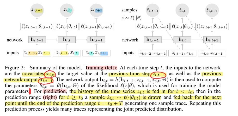
based on Autoregressive Recurrent Network architecture

model distribution : \(Q_{\Theta}\left(\mathbf{z}_{i, t_{0}: T} \mid \mathbf{z}_{i, 1: t_{0}-1}, \mathbf{x}_{i, 1: T}\right)\)

• factorized as

  \(Q_{\Theta}\left(\mathbf{z}_{i, t_{0}: T} \mid \mathbf{z}_{i, 1: t_{0}-1}, \mathbf{x}_{i, 1: T}\right)=\prod_{t=t_{0}}^{T} Q_{\Theta}\left(z_{i, t} \mid \mathbf{z}_{i, 1: t-1}, \mathbf{x}_{i, 1: T}\right)=\prod_{t=t_{0}}^{T} \ell\left(z_{i, t} \mid \theta\left(\mathbf{h}_{i, t}, \Theta\right)\right)\).

• \(\mathbf{h}_{i, t}=h\left(\mathbf{h}_{i, t-1}, z_{i, t-1}, \mathbf{x}_{i, t}, \Theta\right)\).

Information about the observations in the conditioning range \(\mathbf{z}_{i, 1: t_{0}-1}\)

is transferred to the prediction range through the initial state \(\mathbf{h}_{i, t_{0}-1}\)

Given the model parameters \(\Theta\)…

can obtain joint samples \(\tilde{\mathbf{z}}_{i, t_{0}: T} \sim\) \(Q_{\Theta}\left(\mathbf{z}_{i, t_{0}: T} \mid \mathbf{z}_{i, 1: t_{0}-1}, \mathbf{x}_{i, 1: T}\right)\) via ancestral sampling

• step 1) obtain \(\mathbf{h}_{i, t_{0}-1}\) by \(\mathbf{h}_{i, t}=h\left(\mathbf{h}_{i, t-1}, z_{i, t-1}, \mathbf{x}_{i, t}, \Theta\right)\)
  • for \(t=1,...,t_0\)
• step 2) sample \(\tilde{z}_{i, t} \sim \ell\left(\cdot \mid \theta\left(\tilde{\mathbf{h}}_{i, t}, \Theta\right)\right)\)
  • for \(t=t_0,...T\)
  • where \(\tilde{\mathbf{h}}_{i, t}=h\left(\mathbf{h}_{i, t-1}, \tilde{z}_{i, t-1}, \mathbf{x}_{i, t}, \Theta\right)\)

\(\rightarrow\) samples can be used to compute quantities of interests ( ex. quantile )

(1) Likelihood model

two choices :

• 1) (real-valued) Gaussian
• 2) (count data) Negative-binomial

a) Gaussian

mean and standard deviation, \(\theta=(\mu, \sigma)\)

\(\begin{aligned} \ell_{\mathrm{G}}(z \mid \mu, \sigma) &=\left(2 \pi \sigma^{2}\right)^{-\frac{1}{2}} \exp \left(-(z-\mu)^{2} /\left(2 \sigma^{2}\right)\right) \\ \mu\left(\mathbf{h}_{i, t}\right) &=\mathbf{w}_{\mu}^{T} \mathbf{h}_{i, t}+b_{\mu} \quad \text { and } \quad \sigma\left(\mathbf{h}_{i, t}\right)=\log \left(1+\exp \left(\mathbf{w}_{\sigma}^{T} \mathbf{h}_{i, t}+b_{\sigma}\right)\right) \end{aligned}\).

b) Negative-binomial

mean \(\mu \in \mathbb{R}^{+}\)and a shape parameter \(\alpha \in \mathbb{R}^{+}\)

\(\begin{aligned} \ell_{\mathrm{NB}}(z \mid \mu, \alpha) &=\frac{\Gamma\left(z+\frac{1}{\alpha}\right)}{\Gamma(z+1) \Gamma\left(\frac{1}{\alpha}\right)}\left(\frac{1}{1+\alpha \mu}\right)^{\frac{1}{\alpha}}\left(\frac{\alpha \mu}{1+\alpha \mu}\right)^{z} \\ \mu\left(\mathbf{h}_{i, t}\right) &=\log \left(1+\exp \left(\mathbf{w}_{\mu}^{T} \mathbf{h}_{i, t}+b_{\mu}\right)\right) \quad \text { and } \quad \alpha\left(\mathbf{h}_{i, t}\right)=\log \left(1+\exp \left(\mathbf{w}_{\alpha}^{T} \mathbf{h}_{i, t}+b_{\alpha}\right)\right) \end{aligned}\).

(2) Training

given data

• 1) \(\left\{\mathbf{z}_{i, 1: T}\right\}_{i=1, \ldots, N}\)
• 2) associated covariates \(\mathbf{x}_{i, 1: T}\)

optimize parameters \(\Theta\) by maximizing log-likelihood :

• \(\mathcal{L}=\sum_{i=1}^{N} \sum_{t=t_{0}}^{T} \log \ell\left(z_{i, t} \mid \theta\left(\mathbf{h}_{i, t}\right)\right)\).

(3) Scale Handling

Problem : data that shows power-law of scales as…

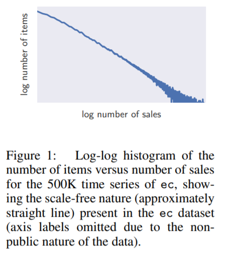
Two problems caused by this :

Problem 1

• network has to learn to scale the input & then invert this scaling at the output

Solution 1

• divide the autoregressive inputs \(z_{i,t}\) ( or \(\tilde{z_{i,t}}\) ) by item-dependent scale factor \(\nu_i\)
• multiply the scale-dependent likelihood params by the same factor
• ex) for Neg-binom…
  • \(\mu=\nu_{i} \log \left(1+\exp \left(o_{\mu}\right)\right)\).
  • \(\alpha=\log \left(1+\exp \left(o_{\alpha}\right)\right) / \sqrt{\nu_{i}}\).
  • where \(o_{\mu}, o_{\alpha}\) are outputs of NN
• for real-valued data, just normalize in advance!

Problem 2

• imbalance in the data

  \(\rightarrow\) stochastic optimization procedure visit small number time-series with a large scale very infrequently

Solution 2

• sample the examples non-uniformly during training
• probability of selecting a window from an example with scale \(\nu_i\) is proportional to \(\nu_i\)

(4) Features

covariates \(\mathbf{x_{i,t}}\) can be item-dependent/independent