Probabilistic Forecasting with Temporal Convolutional Neural Network (2020)

Abstract
Introduction
1. Classical forecasting methods
2. DL based methods
3. Dilated causal convolutional architectures
4. Auto vs Non-Autoregressive
5. (proposal) DeepTCN
Method
1. NN architecture
2. Encoder : Dilated Causal Convolutions
3. Decoder : Residual Neural Network
4. Probabilistic forecasting framework
5. Input Features

0. Abstract

probabilistic forecasting, baed on CNN

under both 1) parametric and 2) non-parametric settings
stacked residual blocks, based on dilated causal convolutional nets
able to learn complex patterns, such as seasonality, holiday effects

1. Introduction

instead of predicting individual/small number of t.s…

\(\rightarrow\) needs to predict thousands/millions of related t.s

1) Classical forecasting methods

ARIMA (Autoregressive Integrated Moving Average)
exponential smoothing ( for univariate base-level forecasting )
ARIMAX = ARIMA + eXogeneous variable

\(\rightarrow\) however, working with thousands/millions of series requires prohibitive labor and computing resources for parameter estimation & not applicable when historical data is sparse / unavailable

2) DL based methods

RNN
Seq2Seq
GRU

\(\rightarrow\) BPTT hampers efficient computations

3) Dilated causal convolutional architectures

Wavenet : alternative for modeling sequential data
staking layers of DCC … receptive fields can be increased

( w.o violating temporal orders )
can be performed in parallel

4) Auto vs Non-Autoregressive

Autoregressive models

ex) seq2seq, wavenet
factorize the joint distn
one-step-ahead prediction approach

Non-Autoregressive models

direct prediction strategy
usually better performances
avoid error accumulation
can be parallelized

5) (proposal) DeepTCN

Deep Temporal Convolutional Network

non-autoregressive probabilistic forecasting
Contributions
- 1) CNN-based forecasting framework
- 2) high scalability & extensibility
- 3) very flexible & include exogenous covariates
- 4) both point & probabilistic forecasting

2. Method

Notation

\(\mathbf{y}_{1: t}=\left\{y_{1: t}^{(i)}\right\}_{i=1}^{N}\) : set of time series ( Multivariate…number of time series \(N\) )
\(\mathbf{y}_{(t+1):(t+\Omega)}=\left\{y_{(t+1):(t+\Omega)}^{(i)}\right\}_{i=1}^{N}\) : future time series
- \(t\) : length of historical observations
- \(\Omega\) : length of forecasting horizon
goal : model the conditional distribution of the future time series \(P\left(\mathbf{y}_{(t+1):(t+\Omega)} \mid \mathbf{y}_{1: t}\right)\)

1) Classical generative models

factorize the joint probability
\(P\left(\mathbf{y}_{(t+1):(t+\Omega)} \mid \mathbf{y}_{1: t}\right)=\prod_{\omega=1}^{\Omega} p\left(\mathbf{y}_{t+\omega} \mid \mathbf{y}_{1: t+\omega-1}\right)\).
challenges
- 1) efficiency issue
- 2) error accumulation

2) Our framework

joint distn DIRECTLY
- \(P\left(\mathbf{y}_{(t+1):(t+\Omega)} \mid \mathbf{y}_{1: t}\right)=\prod_{\omega=1}^{\Omega} p\left(\mathbf{y}_{t+\omega} \mid \mathbf{y}_{1: t}\right)\).
important to allows covariates \(X_{t+\omega}^{(i)}\) (where \(\omega=1, \ldots, \Omega\) and \(\left.i=1, \ldots, N\right)\) t
- \(P\left(\mathbf{y}_{(t+1):(t+\Omega)} \mid \mathbf{y}_{1: t}\right)=\prod_{\omega=1}^{\Omega} p\left(\mathbf{y}_{t+\omega} \mid \mathbf{y}_{1: t}, X_{t+\omega}^{(i)}, i=1, \ldots, N\right)\).
challenge : How to design NN that incorporate historical observations \(\mathbf{y}_{1: t}\) & covariates \(X_{t+\omega}^{(i)}\)

2-1. NN architecture

use both information… \(y_{t}^{(i)}=\nu_{B}\left(X_{t}^{(i)}\right)+n_{t}^{(i)}\).

1) past observation
2) exogenous variables

to extend dynamic regression to multiple t.s forecasting scenario…

\(\rightarrow\) propose a variant of residual NN

Main difference from original ResNet : new block allows for 2 inputs

1) one for historical observation
2) one for exogenous variables

propose DeepTCN

high-level architecture is similar to Seq2Seq framework

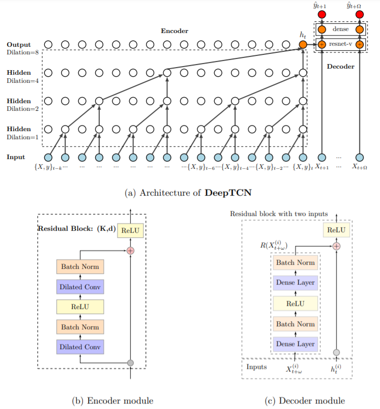
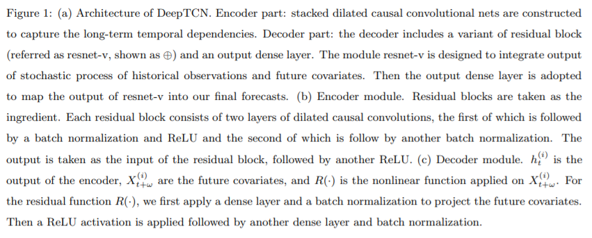
2-2. Encoder : Dilated Causal Convolutions

use inputs, no later than \(t\)
use skipping
notation : \(s(t)=\left(x *_{d} w\right)(t)=\sum_{k=0}^{K-1} w(k) x(t-d \cdot k)\).
stacking multiple Dilated Causal Convolutions :
- enable networks to have very LARGE receptive fields &
- capture LONG-range temporal dependencies with smaller number of layers
Figure 1-a)
- \(d\) =\(\{1,2,4,8\}\)
- \(K\)=2
- receptive filed of size \(16\)

2-3. Decoder : Residual Neural Network

decoder includes 2 parts..

1) variant of residual neural network ( = resnet-v )
2) dense layer
- maps output of 1) into probabilistic forecast
notation : \(\delta_{t+\omega}^{(i)}=R\left(X_{t+\omega}^{(i)}\right)+h_{t}^{(i)}\)
- \(h_{t}^{(i)}\) : latent output of encoder
- \(X_{t+\omega}^{(i)}\) : future covariates
- \(\delta_{t+\omega}^{(i)}\) : latent output of resnet-v
- \(R(\cdot)\) : residual function
output dense layer maps the latent variable \(\delta_{t+\omega}^{(i)}\) to produce the final output \(Z\)

( = probabilistic estimation of interest )

2-4. Probabilistic forecasting framework

output dense layer produce \(m\) outputs : \(Z=\left(z^{1}, \ldots, z^{m}\right)\)
- 2 outputs : ( mean & std ) \(Z_{t+\omega}^{(i)}=\left(\mu_{t+\omega}^{(i)}, \sigma_{t+\omega}^{(i)}\right)\).
probabilistic forecast : \(P\left(y_{t+\omega}^{(i)}\right) \sim G\left(\mu_{t+\omega}^{(i)}, \sigma_{t+\omega}^{(i)}\right)\).

1) Non-parametric approach

forecasts can be obtained by quantile regression
quantile loss : \(L_{q}\left(y, \hat{y}^{q}\right)=q\left(y-\hat{y}^{q}\right)^{+}+(1-q)\left(\hat{y}^{q}-y\right)^{+}\)
- where \((y)^{+}=\max (0, y)\) and \(q \in(0,1)\)
minimize the total quantile loss :
- \(L_{Q}=\sum_{j=1}^{m} L_{q_{j}}\left(y, \hat{y}^{q_{j}}\right)\).

2) Parametric approach

MLE (Maximum Likelihood Estimation)
loss function : negative log-likelihood

\(\begin{aligned} L_{G} &=-\log \ell(\mu, \sigma \mid y) \\ &=-\log \left(\left(2 \pi \sigma^{2}\right)^{-1 / 2} \exp \left[-(y-\mu)^{2} /\left(2 \sigma^{2}\right)\right]\right) \\ &=\frac{1}{2} \log (2 \pi)+\log (\sigma)+\frac{(y-\mu)^{2}}{2 \sigma^{2}} \end{aligned}\).

2-5. Input Features

2 kinds of input features

1) time DEPENDENT
- ex) product price, day of week
2) time INDEPENDENT
- ex) product id, product brand, category

To capture seasonality..

use “hour-of-the day, day-of-the-week….”

Twitter Facebook LinkedIn

(paper) Probabilistic Forecasting with Temporal Convolutional Neural Network

Seunghan Lee